Showing posts with label Group Theory. Show all posts

Tuesday, December 29, 2020

Anatomy of the Pauli Group

Elaboration on Hadamard and Friends - Constructing the Pauli group as the central product of the cyclic group of order four and the dihedral group of a square - Finite group representation and operations in Java.

Introduction


In our previous post about quantum computing, Hadamard and Friends, we touched upon the Pauli group, a group of matrices over the complex domain that represents a collection of elementary quantum gates.

The wikipedia page on the Pauli group states that the group is isomorphic to the central product of the cyclic group of order four and the dihedral group of a square. In this post, we will create representations of various of these groups in Java and demonstrate the isomorphism for \(G_1\), the Pauli group on a single qubit.

Generating the Pauli Group


The Pauli group can be defined using three matrices over the complex domain: $$X=\begin{bmatrix}0&1\\1&0\end{bmatrix},\,Y=\begin{bmatrix}0&-i\\i&0\end{bmatrix},\,Z=\begin{bmatrix}1&0\\0&-1\end{bmatrix}.$$ Before you continue, note that the wikipedia page on Pauli matrices describes a lot of properties and applications of these matrices.

Generating the group using these generators, as illustrated in Generation of a Group, gives us a total of 16 elements: $$\begin{align}G_1=\{\,&X,\,Y,\,Z,\,XX,\,XY,\,XZ,\,YX,\,YZ,\,ZX,\,ZY,\\&XYX,\,XYZ,\,XZX,\,XZY,\,YXY,\,XYXY\,\}.\end{align}$$ The generation of the group can be illustrated using a Cayley graph:
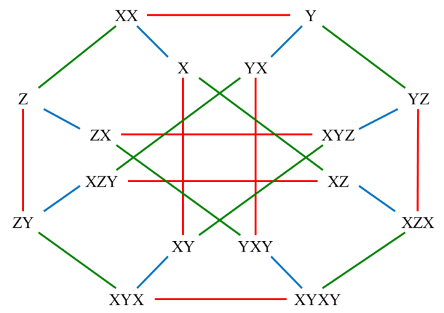
The Cayley Graph for the Generated Pauli Group

Here, multiplication with \(X\), \(Y\) and \(Z\) are represented by a blue, red and green line respectively.

Note that all three generators \(X\), \(Y\) and \(Z\) are their own inverse. For example $$YY=\begin{bmatrix}0&-i\\i&0\end{bmatrix}\begin{bmatrix}0&-i\\i&0\end{bmatrix}=\begin{bmatrix}1&0\\0&1\end{bmatrix}=I.$$ This implies that all operations in the Cayley graph are symmetrical. We therefore use no arrows in the Cayley graph, and any edge can be used in both directions. As another consequence, the neutral element \(I\) is represented as \(XX\).

Each element of the group can be represented in many different ways. For example, it is easy to observe the following equations in the Cayley graph: $$XYZ=YZX=ZXY.$$ The generation process implicitly checks for equal matrices. The notation of the elements above is merely depending on the order in which the generators are combined. The first time a new matrix is obtained, it is added to the set, while subsequent occurrences of the same matrix will not be added to the set.

Enumerating the Pauli Group


The Pauli group can also be defined by enumeration of all elements, using the identity matrix and the generator matrices introduced earlier, multiplied by one of a number of complex factors: $$G_1=\{fA,f\in\{\pm 1,\pm i\},A\in\{I,X,Y,Z\}\}.$$ Consider the matrix multiplication $$XY=\begin{bmatrix}0&1\\1&0\end{bmatrix}\begin{bmatrix}0&-i\\i&0\end{bmatrix}=\begin{bmatrix}i&0\\0&-i\end{bmatrix}=iZ.$$ It is easy to verify that each element of the generated definiton of the group can be written as an element of the enumerated definition of the group. As such, the enumerated group is identical to the generated group. We intentionally do not use the term isomorphic, as the matrices in both groups are identical and the difference is merely in naming.

We can therefore rename the nodes in the Cayley graph based on this enumeration:

The Cayley Graph for the Enumerated Pauli Group

Alternative Generators


Using the Cayley graph, one can observe the symmetry of the generators, in the sense that an even permutation of the generators will not change the structure of the Cayley graph. An even permutation of \(X\), \(Y\) and \(Z\) still yields a correct Cayley graph, where the edges duly represent matrix multiplications. Odd permutations however would require some nodes to trade places in order for the group to be correctly represented.

Looking at the way the group is generated by the three generators, each combination of two generators will generate exactly half of the group. In fact, that is the case for any pair of independent elements of the group.

Applying the generators one after the other, alternatingly, enumerates half of the group in a loop. The third generator is required to get to the other half of the group, where the same loop structure occurs. In fact, that is the case for any combination of generators of the group.

We will now move on to an alternative construction of the Pauli group, as the central product of the cyclic group of order four and the dihedral group of a square.

The Cyclic Group of Order Four


The cyclic group of order 4 is a group with one generator that yields the identity after 4 applications. It can be defined as the additive group of integers modulo 4: $$C_4=\mathbb{Z}/4\mathbb{Z}=\{0,1,2,3\}.$$ Note that a number refers to the equivalence class of that number in the quotient group here.

As we can only represent finite groups, we cannot use the definition based on a quotient group of \(\mathbb{Z}\). We will be using the finite set of integers modulo 4 and define the addition operation on that set, as illustrated in Cyclic Groups.

The Cayley graph for the group is

The Cayley Graph for the Cyclic Group of Order 4

In what follows, we will need the center of \(C_4\). The center of a group is defined as the set of elements that commute with every element in the group. The center of a group \(G\) is denoted and defined by $$Z(G)=\{z\in G|\forall g\in G, zg=gz\}.$$ As \(C_4\) is an Abelian group, its center is the group itself: $$Z(C_4)=C_4=\{0,1,2,3\}.$$ Note that we could just as well create a cyclic group of order 4 using for example the matrix representation of a 90 degrees rotation as a generator. Borrowing on the notation of the Pauli matrices, that would be using the matrix $$R=XZ=\begin{bmatrix}0&1\\1&0\end{bmatrix}\begin{bmatrix}1&0\\0&-1\end{bmatrix}=\begin{bmatrix}0&-1\\1&0\end{bmatrix}.$$ The group would then be defined as the set $$C_4=\{I,R,R^2,R^3\},$$ with composition (matrix multiplication) as an operation.

Note that we could have used any combination of two generators of the Pauli group, in any order, as they will all cycle after four applications. Defining \(R\) as \(XZ\) is just an example with an intuitive meaning.

We could use the matrix representation of \(C_4\) to continue. However, we opted for the integers modulo 4, just to illustrate using groups with different types of elements in our constructions.

The Dihedral Group of a Square


A dihedral group is the symmetry group of a regular polygon. In this case, we need the dihedral group of a square, denoted \(D_8\) in abstract algebra, denoted \(D_4\) in geometry. The group can be generated using two generators: a rotation over 90 degrees, denoted R, and mirroring against the verical axis, denoted M.

We can represent those generators by matrices once more, as transformations in a plane: $$M=\begin{bmatrix}1&0\\0&-1\end{bmatrix},\,R=\begin{bmatrix}0&-1\\1&0\end{bmatrix}.$$ Generating the group using these generators, as illustrated in Generation of a Group, gives us a set of 8 elements: $$D_8=\{I,R,RR,RRR,M,RM,RRM,MR\}.$$ with composition (matrix multiplication) as an operation.

The Cayley graph for this group is

The Cayley Graph for the Dihedral Group of a Square

A red arrow represents multiplication by \(R\), a blue line represents multiplication by \(M\). As before, as \(M\) represents a symmetric operation, the arrows for that generator have been left out.

In what follows, we will need \(Z(D_8)\), the center of \(D_8\). As illustrated in The Center of a Group, we get $$Z(D_8)=\{I,RR\}.$$ That is, besides the identity, \(RR\) is the only element that commutes with every other element in the group.

Note that our center is isomorphic to the cyclic group of order 2: $$Z(D_8)\cong C_2.$$

The Central Product


On the Wikipedia page on the Pauli group, we read that the Pauli group is isomorphic to the central product of the cyclic group of order four and the dihedral group of a square: $$G_1\cong C_4\circ D_8.$$ As a reminder, the Wikipedia page on the central product states that the central product is similar to the direct product, but in the central product two isomorphic central subgroups of the smaller groups are merged into a single central subgroup of the product.

The Direct Product


The set of elements of the direct product of \(C_4\) and \(D_8\) is the cartesian product of the factor groups: $$C_4\times D_8 = \{(n, A)\,|\,n\in C_4, A\in D_8\}.$$ The operation for the direct product is the pairwise application of the operations of the factor groups. Assuming that \(+\) is the group operation of \(C_4\), being the additive group of integers modulo 4, matrix multiplication in \(D_8\) is denoted by juxtaposition, and \(\times\) is the group operation of the direct product, we get: $$(n, A)\times (m, B) = (n+m, AB).$$

The Common Center


Looking at the centers of \(C_4\) and \(D_8\), it is easy to see that the maximum subgroup they have in common is isomorphic to \(C_2\), the cyclic group of order 2. Formulated over the respective alphabets, we get $$\{0, 2\}\cong\{I, RR\}\cong C_2.$$ We will therefore express the commonality using the subgroup \(Z\) of the direct product isomorphic to the common center of the factor groups as: $$Z=\{(0, I), (2, RR)\}\cong C_2.$$ Clearly, \((0, I)\) is the neutral element of the direct product, and consequently also of \(Z\). We quickly verify the cyclic nature of \(Z\), for illustration: $$(2, RR)\times (2, RR) = (2+2, RRRR) = (0, I).$$

An Alternative Definition of the Pauli Group


Now, finally, we are ready to try constructing our alternative Pauli group, as a quotient group we will refer to as \(F_1\), dividing the direct product by the subgroup \(Z\): $$G_1\cong F_1=(C_4\times D_8)/Z.$$ Although we did use the notion of a quotient group already talking about the set of integers modulo 4, we quickly repeat the definiton of a quotient group as given on Wikipedia: $$G/N=\{gN\,|\,g\in G\},$$ where \(G\) is a group and \(N\) is a normal subgroup. Here, \(gN\) is referred to as a coset of \(N\) in \(G\). Typically, different elements \(g\) will result in the same coset when applied to \(N\).

However, for simplicity in notation, for the representation of the quotient group, we will use a representative of each coset rather than the coset iself. For example, we will use \((1, M)\) as the representative of its coset $$(1, M)\times Z=\{(1, M), (3, RRM)\}$$ As such, and as illustrated in The Central Product, we get the following enumeration for the quotient group: $$\begin{align}F_1=\{&(0,I), (0,R), (0,M), (0,RR), (0,RM), (0,MR), (0,RRR), (0,RRM),\\&(1,I), (1,R), (1,M), (1,RR), (1,RM), (1,MR), (1,RRR), (1,RRM)\}\end{align}$$ So far so good, but is this group \(F_1\) really isomorphic to the Pauli group ?

Finding the Isomorphism


To verify whether \(F_1\) is isomorphic to \(G_1\), we have to find a bijection \(\phi\) between the elements of both groups that preserves the group operation. That is, for \(A\) and \(B\) elements of \(G_1\): $$\phi(AB)=\phi(A)\times\phi(B).$$ First of all, the number of elements is fine: \(F_1\) has 16 elements, just as the Pauli group. However, the remainder of the exercise is a bit harder.

We can restrict ourselves to defining the bijection for the generators only, and then verifying preservation of the operation on all combinations (including repetitions) of the generators.

Candidate mappings for the generators should respect a number of constraints. First of all, the identity element can be excluded. Secondly, all generators should be their own inverse, as is the case for \(X\), \(Y\) and \(Z\). This reduces the candidate set to seven elements: $$\{(0,M), (0,RR), (0,RM), (0,MR), (0,RRM), (1,R), (1,RRR)\}$$ Furthermore, logic dictates that in our combination of three generators, all basic building blocks should be represented, in particular the elements \(0\), \(1\), \(R\) and \(M\) of the respective factor groups. This leaves \(2\times 4\times 5=40\) possible combinations of three, ignoring order.

In the java section on Finding an Isomorphism, we do an exhaustive scan, mapping \(X\), \(Y\) and \(Z\) onto different combinations of elements of \(F_1\). Here, we limit ourselves to presenting one of the resulting isomorphisms: $$\phi(X)=(0, M),\,\phi(Y)=(0, RM),\,\phi(Z)=(1, R).$$ Once we have the bijection defined for the generators, the entire group structure follows nicely. This is illustrated once again by a Cayley diagram, the equivalent of the ones presented earlier, but now over our new alphabet:

The Cayley Graph for the Central Product

Note that many more mappings are possible to define the isomorphism, given the symmetries of the Pauli group, and the one presented here represents just one possiblity.

Conclusions


We verified exhaustively that the Pauli group on a single qubit, typically defined as the group generated by three 2x2 matrices over the complex domain, is isomorphic to the central product of the cyclic group of order four and the dihedral group of a square. There's no magic involved here.

Java Implementation


However, the fun in this post is found in the way finite groups can be represented in Java, using whatever type of element and operation that suits the purpose. In addition, constructs such as the direct product, the center and the quotient of groups can be implemented generically on these groups. In what follows, we will illustrate this implementation in Java.

Group Representation


We start our implementation in Java with the definition of the interface that defines a group:
public interface Group<T> {

	public Set<T> getElements();
	public T getIdentity();
	public T multiply(T a, T b);

}

It is defined as a generic interface, where the element type is a parameter. We do not impose any explicit type for the elements of a group, merely that the element type implements equals and hashcode.

A group should be able to produce its elements, as a Java Set, it provides access to the neutral element, and it implements the group operation, referred to as mul.

Note that the group operation could be implemented on the element as well, but that would require an explicit element type, which strongly reduces the genericity of the group implementation.

Also note that we did not include the concepts of symmetric elements, as we do not need them in the scope of this post. We are confident that this could be added to the implementation without breaking the approach taken.

Enumeration of a Group


As a first implementation of the group interface we will focus on an enumerated group:
public class EnumeratedGroup<T> implements Group<T> {

    private Set<T> elements;
    private T identity;
    private BiFunction<T, T, T> operation;

    public EnumeratedGroup(Set<T> elements, T identity, BiFunction<T, T, T> operation) {
        this.elements = new HashSet<>(elements);
        this.identity = identity;
        this.operation = operation;
    }

    ...

    @Override
    public T multiply(T a, T b) {
        return operation.apply(a, b);
    }

}

The constructor of the group requires the set of elements of the group, an explicit reference to the identity element, and a binary function that implements the group operation.

The implementation of this class is straightforward now. You will want to add getters and at least provide an implementation for toString. We only included the implementation of the multiply function, just in case.

Generation of a Group


Next comes the implementation of a group specified using a finite set of generators:
public class GeneratedGroup<T> implements Group<T> {

    private Set<T> generators;
    private Set<T> elements;
    private T identity;
    private BiFunction<T, T, T> operation;

    public GeneratedGroup(Set<T> generators, T identity, BiFunction<T, T, T> operation) {
        this.generators = generators;
        this.identity = identity;
        this.operation = operation;
    }

    @Override
    public Set<T> getElements() {
        if (elements==null) {
            elements = new HashSet<>(generators);
            elements.add(getIdentity());
            int size = 0;
            while (size<elements.size()) {
                size = elements.size();
                Set<T> generated = new HashSet<>();
                for (T t : elements) {
                    for (T g : generators) {
                        generated.add(multiply(t, g));
                    }
                }
                elements.addAll(generated);
            }
        }
        return elements;
    }

    ...

}

Again, simple implementation details are left out.

The thing worth mentioning here is the getElements function, implemented lazily. On first invocation, it will generate the set of elements based on the identity element and the set of generators using a fixed point approach:
  • We start with the set of elements consisting of the identity element only.
  • We then keep applying all generators to all elements of this set, and adding these as new elements, until the set no longer grows in size.

The Pauli Group


We now have sufficient building blocks to implement a first version of the Pauli group, with matrices as elements, using generators. We will be using the matrices introduced in Generating the Pauli Group.

We will be borrowing the matrix implementation of our previous post about quantum computing, Hadamard and Friends. And we have an alphabet of matrices ready:
public class Alphabet {

    public static final Matrix I = MatrixUtils.identity(2);

    public static final Matrix X = new Matrix("X", new Double[][] { { 0d, 1d }, { 1d, 0d } });
    public static final Matrix Y = new Matrix("Y", new Double[][] { { 0d, -1d }, { 1d, 0d } }).cmul(Complex.I).setName("Y");
    public static final Matrix Z = new Matrix("Z", new Double[][] { { 1d, 0d }, { 0d, -1d } });

    ...

}

Multi-dimensional complex array constants are cumbersome to write, and the Matrix implemention is immutable. Therefore, we have to rename the matrix \(Y\) after multiplication with the complex number \(i\).

The Pauli group can now easily be defined as:
public class GroupUtils {

    public static Group<Matrix> getPauliGroup() {
        Set<Matrix> generators = new HashSet<>(Arrays.asList(Alphabet.X, Alphabet.Y, Alphabet.Z));
        return new GeneratedGroup<Matrix>(generators, Alphabet.I, (a, b) -> a.vmul(b));
    }

    ...

}

Cyclic Groups


For the alternative implementation of the pauli group, we first need a cyclic group of order four. We cannot define this group as the quotient \(\mathbb{Z}/4\mathbb{Z}\), as we can only handle finite groups. We will therefore explicitly define modulo numbers and once more use a generated group.
public class Modulo {

    private int value;
    private int modulo;

    public Modulo(int value, int mod) {
        this.value = value%mod;
        this.modulo = mod;
    }

    public Modulo add(Modulo m) {
        return new Modulo(value+m.getValue(), modulo);
    }

    ...

}

Completing the implementation is straightforward. We added the implementation of the group operation add, just in case.

The cyclic group of order four can now be easily defined as:
public class GroupUtils {

    public static Group<Modulo> getCyclicGroup(int size) {
        HashSet<Modulo> generators = new HashSet<>(Arrays.asList(new Modulo(1, size)));
        return new GeneratedGroup<Modulo>(generators, new Modulo(0, size), (a, b) -> a.add(b));
    }

    ...

}

The Dihedral Group of Order Eight


The dihedral group of order eight can equally be defined as a generated group, using the matrices introduced in The Dihedral Group of a Square. Therefore, this section is very similar to the one where we introduced the matrix representation of The Pauli Group.

First we need the matrix definitions:
public class Alphabet {

    public static final Matrix R = new Matrix("R", new Double[][] { { 0d, -1d }, { 1d, 0d } });
    public static final Matrix M = new Matrix("M", new Double[][] { { 1d, 0d }, { 0d, -1d } });

    ...

}

Then we are ready to create the group:
public class GroupUtils {

    public Group<Modulo> getDihedral8Group() {
        Set<Matrix> generators = new HashSet<>(Arrays.asList(Alphabet.R, Alphabet.M));
        return new GeneratedGroup<Matrix>(generators, Alphabet.I, (a, b) -> a.vmul(b));
    }

    ...

}

The Center of a Group


Comes the time we need to compute the center of a group:
public class GroupUtils {

    public static <T> Group<T> getCenter(Group<T> group) {
        Set<T> center = group.getElements().stream()
            .filter(z -> group.getElements().stream()
                .filter(g -> !group.multiply(z, g).equals(group.multiply(g, z))).count()==0l)
            .collect(Collectors.toSet());
        return new EnumeratedGroup<T>(center, group.getIdentity(), group::multiply);
    }

    ...

}

We provide a stream style implementation, that filters all elements of the group (the outer filter) that commute with all elements of the group (the inner filter) to determine the elements of the center. We then use that set to create an enumerated group with the same identity element and the same group operation.

The Direct Product


By now, the exercise risks becoming just more of the same thing. We can implement the direct product of two groups as the Cartesian product of the elements in the group with the pairwise group operations.
public class ProductGroup<T, S> implements Group<Pair<T, S>> {

    private Group<T> tgroup;
    private Group<S> sgroup;
    private Set<Pair<T, S>> elements;

    public ProductGroup(Group<T> tgroup, Group<S> sgroup) {
        this.tgroup = tgroup;
        this.sgroup = sgroup;
    }

    @Override
    public Set<Pair<T, S>> getElements() {
        if (elements==null) {
            elements = new HashSet<>();
            for (T t : tgroup.getElements()) {
                for (S s : sgroup.getElements()) {
                    elements.add(new Pair<>(t, s));
                }
            }
        }
        return elements;
    }

    @Override
    public Pair<T, S> getIdentity() {
        return new Pair<>(tgroup.getIdentity(), sgroup.getIdentity());
    }

    @Override
    public Pair<T, S> multiply(Pair<T, S> a, Pair<T, S> b) {
        return new Pair<>(tgroup.multiply(a.getT(), b.getT()), sgroup.multiply(a.getS(), b.getS()));
    }

    ...

}

We us a Pair to combine two elements, one of each group. You can use any implementation you can find, or write your own. Just make sure to implement equals and hashcode in a proper way.

Again we have a lazy implementation of the getElements method that calculates the Cartesian product of the elements of the two groups as a set of pairs. The identity element is the pair of the identity elements of both groups. The operation is the pairwise multiplication of the elements of both groups.

Quotient Groups


The implementation of a quotient group however is a bit trickier:
public class QuotientGroup<T> implements Group<T> {

    private Group<T> group;
    private Set<T> subgroup;
    private Set<T> elements;
    private Map<T, Set<T>> representation;

    public QuotientGroup(Group<T> group, Set<T> subgroup) {
        this.group = group;
        this.subgroup = subgroup;
    }

    @Override
    public Set<T> getElements() {
        if (elements==null) {
            elements = new HashSet<>();
            representation = new HashMap<>();
            Set<Set<T>> cosets = new HashSet<>();
            for (T e : group.getElements()) {
                Set<T> coset = GroupUtils.multiply(group, subgroup, e);
                if (!cosets.contains(coset)) {
                    elements.add(e);
                    representation.put(e, coset);
                    cosets.add(coset);
                }
            }
        }
        return elements;
    }

    @Override
    public T getIdentity() {
        return group.getIdentity();
    }

    private T normalize(T t) {
        T n = GroupUtils.findElement(representation, t);
        if (n!=null) {
            return n;
        }
        return t;
    }

    @Override
    public T multiply(T a, T b) {
        return normalize(group.multiply(a, b));
    }

    ...

}

We start with a group and a subgroup, the latter represented as a set of elements only. In addition to that, the impementation will keep track of the set of elements, as most of the Group implementations. However, as we will represent each coset by a unique representative of the coset, we need to keep track of which element represents which coset. This is done using the representation, a mapping of represtatives to cosets.

As before, the elements are determined lazily. To determine the set of elements, we scan the elements of the larger group and determine the coset of the smaller group for each element. Is this is a new coset, we use the element as a representative for that coset, and update the representation map. If we already have the coset, we replace the element by its representation.

The getElements function uses a utility function GroupUtils.multiply for this purpose, that determines the coset of an element of the group:
public class GroupUtils {

    public static <T> Set<T> multiply(Group<T> group, Set<T> elements, T element) {
        return elements.stream().map(e -> group.multiply(e, element)).collect(Collectors.toSet());
    }

    ...

}

The QuotientGroup implementation has a private member function normalize that does the same thing, replacing an element by its unique representative, that we use after every calculation. For now, that is only in the multiply function. It uses another utility function GroupUtils.findElement, that finds the coset in the representation map that contains a newly created element, and returns the representation of that coset:
public class GroupUtils {

     public static <T> T findElement(Map<T, Set<T>> map, T t) {
        for (T r : map.keySet()) {
            if (map.get(r).contains(t)) {
                return r;
            }
        }
        return null;
    }

    ...

}

The Central Product


We now have sufficient building blocks to implement the second version of the Pauli group, as the central product of the cyclic group of order four and the dihedral group of a square.
public class GroupUtils {

    public static <T> Group<Pair<Modulo, Matrix>> getCentralProductPauliGroup() {
        Group<Modulo> cyclic4 = getCyclicGroup(4);
        Group<Matrix> dihedral8 = getDihedral8Group();
        Group<Pair<Modulo, Matrix>> product = new ProductGroup<>(cyclic4, dihedral8);
        Set<Pair<Modulo, Matrix>> subgroup = getCentralProductPauliSubGroup();
        return new QuotientGroup<>(product, subgroup);
    }

    public static <T> Set<Pair<Modulo, Matrix>> getCentralProductPauliSubGroup() {
        Set<Pair<Modulo, Matrix>> subgroup = new HashSet<>();
        subgroup.add(new Pair<>(new Modulo(0, 4), Alphabet.I));
        subgroup.add(new Pair<>(new Modulo(2, 4), r.vmul(r)));
        return subgroup;
    }

    ...

}

Note that we explicitly construct the subgroup of the direct product isomorphic to the maximum common subgroups of the centers of both factor groups of the direct product. Let's say we leave the generic implementation of that step as an exercise.

Finding an Isomorphism


Verifying whether a mapping between groups is an isomorphism is easy. Assume we represent the isomorphism as a mapping of elements from one group to the other:
public class GroupUtils {

    public static <T, S> boolean isIsomorphism(Group<T> tgroup, Group<S> sgroup, Map<T, S> map) {
        if (tgroup.getElements().size()!=sgroup.getElements().size()) {
            return false;
        }
        for (T a : tgroup.getElements()) {
            for (T b : tgroup.getElements()) {
                if (!map.get(tgroup.multiply(a, b)).equals(sgroup.multiply(map.get(a), map.get(b)))) {
                    return false;
                }
            }
        }
        return true;
    }

    ...

}

If the number of elements in both groups is different, the groups cannot possibly be isomorphic. Otherwise, we just check any combination of two elements of the first group, and verify whether the product of the images of the elements equals the image of the product. Any mismatch will refute the isomorphic character of the mapping.

Finding an isomorphism between two groups is trickier. Suppose we have generators for both groups, then we can gradually construct the isomorphism, and check for inconsistencies along the way:
public class GroupUtils {

    public static <T, S> Map<T, S> getIsomorphism(Group<T> tgroup, Group<S> sgroup, List<T> tgenerators, List<S> sgenerators) {
        if (tgenerators.size()!=sgenerators.size()) {
            return null;
        }
        Map<T, S> isomorphism = new HashMap<>();
        isomorphism.put(tgroup.getIdentity(), sgroup.getIdentity());
        for (int i=0; i<tgenerators.size(); ++i) {
            isomorphism.put(tgenerators.get(i), sgenerators.get(i));
        }
        int size = 0;
        while (isomorphism.size()>size) {
            size = isomorphism.size();
            Map<T, S> mapping = new HashMap<>();
            for (T t1 : isomorphism.keySet()) {
                for (T t2 : isomorphism.keySet()) {
                    T tproduct = tgroup.multiply(t1, t2);
                    S sproduct = sgroup.multiply(isomorphism.get(t1), isomorphism.get(t2));
                    S expected = isomorphism.get(tproduct);
                    if (expected==null) {
                        expected = mapping.get(tproduct);
                    }
                    if (expected==null) {
                        mapping.put(tproduct, sproduct);
                    } else if (!sproduct.equals(expected)) {
                        return null;
                    }
                }
            }
            isomorphism.putAll(mapping);
        }
        return isomorphism;
    }

    ...

}

In what follows we will refer to the first group as the domain of the isomorphism and to the second group as the image of the isomorphism.

We assume that the list of generators that are provided for both groups already reflect the isomorphism. Therefore, they should be of equals size.

Then we initialize the isomorphism with the generators. We then extend the isomorphism by trying all combinations of elements in the domain, and calculating the products of their images and the image of their product. If the product is not yet present in the domain of the isomorphism, we add a mapping. If the product is present already, its image in the isomorphism should be equals to what we just calculated.

Because we cannot iterate over a collection while it is being modified, we accumulate new mappings in a separate data structure. We then merge all new mappings into the isomorphism after all combination of elements in the domain have been processed.

We repeat this process until the isomorphism no longer grows in size, effectively finding a fixed point for the process. Under the assumption that the initial elements provided are generators for the doamin and the image of the isomorphism, respectively, the fixed point will represent an isomorphism between both groups.

We realize this is all a bit messy, but we basically come to the same conclusion as Naftali Harris on this subject: finding an isomorphism between two groups is not a trivial task. However, using generators will reduce the complexity in a significant way.

Selecting Generators


The only step remaining to close the loop here, is finding the generators for the image. We will leave out the coding details, but give you the results.

We already have the generators for the domain, being \(X\), \(Y\) and \(Z\). Starting with all 16 elements of the image, we can limit ourselves to those that are a root of the identity element, as we know this condition holds for the generators of the domain. Excluding the identity itself, we find 7 elements that square to the identity:
[(0,M), (0,RR), (0,RM), (0,MR), (0,RRM), (1,R), (1,RRR)]

If we try each combination of three elements out of this set, no repetition, order matters, we get \(7!/3!=210\) possible combinations. Out of these, it turns out that \(48\) can be used to construct an isomorphism.

Knowing that the group structure is invariant under permutations of those three generators, and there are \(3!=6\) permutations of three elements, we get \(48/6=8\) combinations, ignoring order, that do the job. Here they are:
[
  [(0,M), (0,RM), (1,R)], [(0,M), (0,RM), (1,RRR)],
  [(0,M), (0,MR), (1,R)], [(0,M), (0,MR), (1,RRR)],
  [(0,RM), (0,RRM), (1,R)], [(0,RM), (0,RRM), (1,RRR)],
  [(0,MR), (0,RRM), (1,R)], [(0,MR), (0,RRM), (1,RRR)]
]

Conclusions


Wrapping the standard Java Set interface and its implementations with some additional characteristics provides an easy way to implement finite groups and play around with them. As can be expected however, one quickly gets into the realms of NP-complete problems. For the Pauli group on a single qubit, the limited quantitative complexity helped us to gain some insights.

Wednesday, November 1, 2017

How to Become an Astronaut

On Tim Peake's selection exam to become an astronaut, the group of rotations of a cube, solving the question the long way, using Knuth Bendix Completion.
(updated on 15-06-2020)

Introduction


Recently, Tim Peake tweeted a Friday Night Brain Teaser about a question he was asked when taking the selection examination for admission to the astronaut program. The question was about the capacity for one to imagine 3D manipulations of a cube.

In this post, we will use the results of a previous post on Knuth Bendix Completion to find an answer to the question. No doubt this is not the shortest solution, but it surely is an interesting one.

The Question


Imagine a cube in front of you. The cube can be rolled left and right, and backward and forward. The bottom of the cube is marked with a black dot.


Imagine rolling the cube forward, left, left, forward, right, backward, right. Where is the black dot now ?

The Solution


Although the solution is quite obvious for those of us with good spatial sense, it is interesting to approach the problem from an algebraic view.

In a previous post, we talked about Knuth-Bendix Completion on Non-Abelian Group Theory. As the set of transformations of a cube with composition as an operation is a non-Abelian group, we will unleash the Knuth-Bendix Completion procedure on this group.

If the procedure terminates, we will have a decidable rewrite system that implements this group. We will then apply this rewrite system to find the normal form of the sequence of rotations specified in the question and see what comes out.

Transformations of a Cube


The number of positions, including orientation, of a cube is easy to determine. There are six sides to a cube, and for each side there are four possible orientations. This brings the total number of positions to 24 (6x4).

Imagine a given starting position for a cube. Each of the 24 positions corresponds to a transformation of the cube from the starting position to that position. This gives a collection of 24 transformations that, with composition as an operator, forms a non-Abelian group. This group is referred to as the transformation group of a cube.

Permutations of Four


The Internet is full of sources stating that the group of transformations of a cube is isomorphic to the group of permutations of four elements, referred to as S4. An isomorphism is a one-to-one relationship between the elements of two groups groups that preserves the group operation. We will come back to this property lateron.

Consider an ordered collection of 4 objects, say 1234. Then consider all the possible ways in which these 4 elements can be ordered, called permutations of these 4 objects.

To create such a configuration of 4, we have 4 possiblities for the first position, 3 for the second position (as one object is already used), 2 for the third position and then only one object is left for the fourth position. This gives a total of 24 (4x3x2x1 or 4!) permutations.

Some sources are providing a proof of the isomorphism. We will take a more visual approach.

The Cayley Graph


A Cayley graph visualizes the structure of a group based on a limited number of elements, called generators. The idea is that any element of the group, without exception, can be written as a composition of generators. For the permutation group of four, this gives an interesting diagram:


In the bottom left corner is our starting configuration 1234. A red arrow, representing the rotation to the right, brings us to 4123. A blue arrow, representing the rotation to the left of the 3 leftmost objects while keeping the righmost object in place, brings us to 2314. We will refer to the transformation represented by the red arrow as C, and the transformation represented by the blue arrow as S.

As you can see in the diagram, compositions of only these two generating elements of the group can be used to construct any of the 24 permutations, in various ways. Moreover, C is cyclic after four compositions, resulting in a number of red squares, while S is cyclic after three compositions, resulting in a number of blue triangles. Although the squares are not connected and the triangles are not connected, together, they create a fully connected graph.

Note that the collection of generators is not unique, in the sense that different collections of elements of the group may be used as generators. What's special about this collection is that it results in a nice graphical representation without crossing arrows, which is certainly not always the case.

You will find the Cayley graph and a lot more visuals on the wikiversity page on the Symmetric Group S4.

The Isomorphism


Coming back to the group of transformations of a cube, we could try to find a collection of generators and construct a Cayley diagram. However, as the two groups are isomorphic, with the right representation of the positions of a cube and the right choice of generators, we should get the same Cayley diagram.

First, let's look at the representation of the position of a cube. We will use a dice for this purpose, to easily distinguish between different positions. We will label the corners of the dice with labels 1, 2, 3 and 4, in such a way that each side has four different labels. It turns out that, after choosing the labels for one side, only one possibility is left to complete the labeling for the whole dice:


For the top side of the dice, we choose the labels to start with 1 for the corner closest to us, and continue clockwise while counting to 4, as illustrated by the blue labels. The labels of the corners of the bottom side can then only be chosen equal to the diagonally opposite corner, as illustrated by the red labels (where label 1 is at the back and not shown). The position of the dice when labeling is important, but arbitrary.

We will then represent the position of a cube by enumerating the labels of the corners of the top side, starting with the corner closest to us, and continuing clockwise. This results in the following observations:
  • The representations of all possible positions of a cube correspond exactly with the permutations of four.
  • The transformation represented by C is clockwise rotation around the vertical axis.
  • The transformation represented by S is anti-clockwise rotation around the horizontal axis (front left to back right), followed by clockwise rotation around the vertical axis.

With this representation, the Cayley graph for both groups is identical. Grab a dice and try it out ! And since any element of each group can be written as the same composition of generators, the relation preserves the group operation.

Knuth-Bendix Completion


We are now ready to start solving the question. We will start with the axioms of non-Abelian groups, define constants for the generators and add some axioms related to the generators. Then, Knuth-Bendix Completion will solve the question for us.

The Alphabet


An intuitive alphabet to represent the set of rotations on a cube, besides the identity, consists of a 90° rotation around each axis in 3D-space:
  • R - Right: Rolling the cube around the Y-axis, to the right.
  • C - Clockwise: Rolling the cube around the Z-axis, clockwise.
  • B - Backward: Rolling the cube around the X-axis, towards yourself.

Yes, we added an extra degree of freedom here, to prepare for interplanetary travel, say.

For readability, and because they are used in the question, we will add the inverse operations to the alphabet as well:
  • L - Left: Rolling the cube around the Y-axis, to the left.
  • A - Anti-Clockwise: Rolling the cube around the Z-axis, anti-clockwise.
  • F - Forward: Rolling the cube around the X-axis, away from yourself.

However, we will construct our theory using only the two generators introduced before, defined as:
  • C - Clockwise rotation around the vertical axis (hey, what a coincidence).
  • S - Rotate anti-clockwise around the horizontal axis, followed by rotate clockwise around the vertical axis.

One can easily express the transformations used in the question in function of these generators as follows:
  • R = S*S*C*S
  • L = C*S*S
  • B = S*S*C
  • F = C*C*C*S

Remember, the composition operator reverses the order of operation: C*S reads as "C after S".

The Theory


We will start off with the three axioms of non-Abelian group theory. Closure is implicit.

[1] a*1 = a
[2] a*i(a) = 1
[3] a*b*c = a*(b*c)

Then, we will add a minimum set of axioms defining the interaction of the transformations C and S.
[4] i(C) = C*C*C
[5] i(S) = S*S

Here we express the cyclic character of these transformations, as stated before: C is cyclic after four compositions and S is cyclic after three compositions. Note that these axioms correspond to loops in the Cayley diagram.

Observing the diagram somewhat closer, we notice one other type of loop, involving a combination of red and blue arrows. We add this relationship as an axiom too.
[6] i(C) = S*C*S

This completes our theory. Note that we did not orient the axioms lexicographically, from "complex" to "simple", as mentioned in the post on the Knuth-Bendix Completion procedure. This is not necessary, as the procedure does the orientation by itself.

The Rewrite System


As explained in our previous post on Knuth-Bendix Completion, we will try generating a decidable rewrite system out of this theory. And indeed, after the ninth iteration, a rewrite system is produced consisting of 39 rewrite rules.
[1]  a*1 -> a
[2]  a*i(a) -> 1
[3]  a*b*c -> a*(b*c)
[4]  S*(C*S) -> i(C)
[5]  i(S) -> S*S
[6]  C*(C*C) -> i(C)
[7]  a*(i(a)*b) -> b
[8]  S*(S*S) -> 1
[9]  1*a -> a
[10] S*(C*(S*a)) -> i(C)*a
[11] C*(C*(C*a)) -> i(C)*a
[12] S*(S*(S*a)) -> a
[13] i(C)*i(C) -> C*C
[14] S*(S*i(C)) -> C*S
[15] i(C)*(i(C)*a) -> C*(C*a)
[16] i(C)*(S*S) -> S*C
[17] S*(S*(i(C)*a)) -> C*(S*a)
[18] i(C)*(S*(S*a)) -> S*(C*a)
[19] i(1) -> 1
[20] S*(S*(C*C)) -> C*(S*i(C))
[21] S*(C*(C*S)) -> i(C)*(S*i(C))
[22] S*(S*(C*(C*a))) -> C*(S*(i(C)*a))
[23] C*(S*C) -> S*S
[24] C*(C*(S*S)) -> i(C)*(S*C)
[25] i(b)*(b*a) -> a
[26] i(i(a)) -> a
[27] S*(C*(C*(S*a))) -> i(C)*(S*(i(C)*a))
[28] C*(S*(C*a)) -> S*(S*a)
[29] C*(C*(S*(S*a))) -> i(C)*(S*(C*a))
[30] S*(i(C)*(S*i(C))) -> C*(S*(i(C)*S))
[31] i(C)*(S*(i(C)*S)) -> S*(i(C)*(S*C))
[32] C*(S*(i(C)*(S*C))) -> S*(i(C)*S)
[33] i(a)*a -> 1
[34] S*(i(C)*(S*(i(C)*a))) -> C*(S*(i(C)*(S*a)))
[35] i(C)*(S*(i(C)*(S*a))) -> S*(i(C)*(S*(C*a)))
[36] C*(S*(i(C)*(S*(C*a)))) -> S*(i(C)*(S*a))
[37] i(b*a) -> i(a)*i(b)
[38] S*(i(C)*(S*(C*(C*a)))) -> C*(C*(S*(i(C)*(S*a))))
[39] C*(C*(S*(i(C)*S))) -> S*(i(C)*(S*(C*C)))

The rewrite system has the same expressive power as the theory it originates from, but it has the advantage of decidability: semantic equality of terms can be verified using syntactic equality of normal forms, which are unique and guaranteed to exist.

Rewriting


Comes the time to take the sequence of rotations mentioned in the question and try rewriting it. Taking into account that our composition operator reverses the order of operation, the sequence forward, left, left, forward, right, backward, right should be represented as R*B*R*F*L*L*F. We then substitute the tranformations in this expression by their representation in terms of generators, and rewrite this term:
S*S*C*S*(S*S*C)*(S*S*C*S)*(C*C*C*S)*(C*S*S)*(C*S*S)*(C*C*C*S)
  [3]  -> S*S*C*S*(S*S*C)*(S*S*C*S)*(C*C*C*S)*(C*S*S)*(C*S*S*(C*C*C*S))
  [3]  -> S*S*C*S*(S*S*C)*(S*S*C*S)*(C*C*C*S)*(C*S*S*(C*S*S*(C*C*C*S)))
  [3]  -> S*S*C*S*(S*S*C)*(S*S*C*S)*(C*C*C*S*(C*S*S*(C*S*S*(C*C*C*S))))
  [3]  -> S*S*C*S*(S*S*C)*(S*S*C*S*(C*C*C*S*(C*S*S*(C*S*S*(C*C*C*S)))))
  [3]  -> S*S*C*S*(S*S*C*(S*S*C*S*(C*C*C*S*(C*S*S*(C*S*S*(C*C*C*S))))))
  [3]  -> S*S*C*(S*(S*S*C*(S*S*C*S*(C*C*C*S*(C*S*S*(C*S*S*(C*C*C*S)))))))
  [3]  -> S*S*(C*(S*(S*S*C*(S*S*C*S*(C*C*C*S*(C*S*S*(C*S*S*(C*C*C*S))))))))
  [3]  -> S*(S*(C*(S*(S*S*C*(S*S*C*S*(C*C*C*S*(C*S*S*(C*S*S*(C*C*C*S)))))))))
  [10] -> S*(i(C)*(S*S*C*(S*S*C*S*(C*C*C*S*(C*S*S*(C*S*S*(C*C*C*S)))))))
  [3]  -> S*(i(C)*(S*S*(C*(S*S*C*S*(C*C*C*S*(C*S*S*(C*S*S*(C*C*C*S))))))))
  [3]  -> S*(i(C)*(S*(S*(C*(S*S*C*S*(C*C*C*S*(C*S*S*(C*S*S*(C*C*C*S)))))))))
  [18] -> S*(S*(C*(C*(S*S*C*S*(C*C*C*S*(C*S*S*(C*S*S*(C*C*C*S))))))))
  [23] -> C*(S*(i(C)*(S*S*C*S*(C*C*C*S*(C*S*S*(C*S*S*(C*C*C*S)))))))
  [3]  -> C*(S*(i(C)*(S*S*C*(S*(C*C*C*S*(C*S*S*(C*S*S*(C*C*C*S))))))))
  [3]  -> C*(S*(i(C)*(S*S*(C*(S*(C*C*C*S*(C*S*S*(C*S*S*(C*C*C*S)))))))))
  [3]  -> C*(S*(i(C)*(S*(S*(C*(S*(C*C*C*S*(C*S*S*(C*S*S*(C*C*C*S))))))))))
  [18] -> C*(S*(S*(C*(C*(S*(C*C*C*S*(C*S*S*(C*S*S*(C*C*C*S)))))))))
  [22] -> C*(C*(S*(i(C)*(S*(C*C*C*S*(C*S*S*(C*S*S*(C*C*C*S))))))))
  [3]  -> C*(C*(S*(i(C)*(S*(C*C*C*(S*(C*S*S*(C*S*S*(C*C*C*S)))))))))
  [3]  -> C*(C*(S*(i(C)*(S*(C*C*(C*(S*(C*S*S*(C*S*S*(C*C*C*S))))))))))
  [3]  -> C*(C*(S*(i(C)*(S*(C*(C*(C*(S*(C*S*S*(C*S*S*(C*C*C*S)))))))))))
  [36] -> C*(S*(i(C)*(S*(C*(C*(S*(C*S*S*(C*S*S*(C*C*C*S)))))))))
  [36] -> S*(i(C)*(S*(C*(S*(C*S*S*(C*S*S*(C*C*C*S)))))))
  [10] -> S*(i(C)*(i(C)*(C*S*S*(C*S*S*(C*C*C*S)))))
  [15] -> S*(C*(C*(C*S*S*(C*S*S*(C*C*C*S)))))
  [3]  -> S*(C*(C*(C*S*(S*(C*S*S*(C*C*C*S))))))
  [3]  -> S*(C*(C*(C*(S*(S*(C*S*S*(C*C*C*S)))))))
  [11] -> S*(i(C)*(S*(S*(C*S*S*(C*C*C*S)))))
  [18] -> S*(S*(C*(C*S*S*(C*C*C*S))))
  [3]  -> S*(S*(C*(C*S*(S*(C*C*C*S)))))
  [3]  -> S*(S*(C*(C*(S*(S*(C*C*C*S))))))
  [22] -> C*(S*(i(C)*(S*(S*(C*C*C*S)))))
  [18] -> C*(S*(S*(C*(C*C*C*S))))
  [3]  -> C*(S*(S*(C*(C*C*(C*S)))))
  [3]  -> C*(S*(S*(C*(C*(C*(C*S))))))
  [22] -> C*(C*(S*(i(C)*(C*(C*S)))))
  [25] -> C*(C*(S*(C*S)))
  [28] -> C*(S*(S*S))
  [8]  -> C*1
  [1]  -> C

So, the transformation mentioned in the question is equal to a single rotation around the Z-axis, clockwise. Consequently, the cube will still be positioned on the side with the black dot, albeit rotated by 90°, which is irrelevant for answering the question.

A Note on Expressivity


Admitted, the reduction is quite verbose. This is obviously caused by the fact that we limit our alphabet to the two generators only. A similar exercise where all the 90° rotations and their inverse are added to the alphabet, and the theory is extended with the axioms reflecting their relationships, works equally well, with the desired brevity. However, the rewrite system generated by the Knuth-Bendix completion procedure consists of 92 rewrite rules, as there are a lot more relationships to capture.

We will not present the completed rewrite system over the extended alphabet here, but we do provide the reduction of the term using this extended alphabet:
R*B*R*F*L*L*F
  [3]  -> R*B*R*F*L*(L*F)
  [3]  -> R*B*R*F*(L*(L*F))
  [3]  -> R*B*R*(F*(L*(L*F)))
  [3]  -> R*B*(R*(F*(L*(L*F))))
  [3]  -> R*(B*(R*(F*(L*(L*F)))))
  [33] -> B*(C*(R*(F*(L*(L*F)))))
  [32] -> B*(B*(C*(F*(L*(L*F)))))
  [58] -> A*(B*(B*(F*(L*(L*F)))))
  [55] -> A*(B*(L*(L*F)))
  [49] -> B*(L*F)
  [21] -> B*(C*L)
  [56] -> C

Conclusion


We are going to Mars !

The group of rotations of a cube nicely passes Knuth-Bendix Completion and the resulting rewrite system solves the Friday night brain teaser, mechanically, deterministically, in the blink of an eye.

We cannot be sure of our theory to be true, but it is correct, and, more importantly, it solves the issue.

Saturday, July 22, 2017

Knuth-Bendix Completion on Non-Abelian Group Theory

Applying Knuth-Bendix Completion to the theory of non-abelian groups to come to a rewrite system that reflects decidability of the theory it implements, where semantic equality is equivalent to syntactic equality of normal forms.

Introduction


It turns out that the way we were thought group theory in the lower grades of high school was not optimal, at least not from a computational point of view. Simple statements in group theory could be rather tricky to prove, while some theories are decidable and consequently problems formulated in these theories can be solved mechanically.

In this post, we will use a procedure referred to as Knuth-Bendix completion to transform the traditional axioms for non-abelian group theory into a deterministic rewrite system with the same expressive power. The different steps of the procedure are enumerated exhaustively. Intermediate theories will introduce new axioms and make older ones obsolete.

Being exhaustive makes the post somewhat verbose. In fact, the text has largely been generated as a side effect of the automation of the Knuth-Bendix completion procedure. Skip the sections that feel like you get them. Use them for reference if you are interested in the detail.

The whole Knuth-Bendix completion procedure on non-abelian group theory is presented graphically using the graphviz dot language. Go for the graphics if you want to scan through quickly.

Non-Abelian Groups


A non-abelian group is defined as a collection of elements, a binary operation on these elements and four axioms: closure, identity, invertibility and associativity. We will consider the collection of all well-formed terms over an alphabet using a typical algebraic term syntax, meaning closure is implicit.

The theory of non-abelian groups can then be formulated using the axioms:
[1] a*1 = a
[2] a*i(a) = 1
[3] a*b*c = a*(b*c)
Here, the binary operation is represented by an asterisk (*), and any letter that is not used as a functor denotes a variable.

Briefly explained:
  • Axiom [1] states that there is an element 1 which is the right-side identity for the operation.
  • Axiom [2] states that the unary functor i denotes right-side inverse element of its argument.
  • Axiom [3] expresses that the binary operation is associative. The operation is assumed to associate to the left, but that is mere notational convention.

A Simple Exercise


Semantic equality in non-abelian groups is decidable, meaning that there is an effective procedure to determine semantic equality within finite space and time. However, using the axioms provided above, decidability may not be apparent.

Let's illustrate the problem with a simple exercise, proving that the right-side inverse is also the left-side inverse, a property known to be valid for non-abelian groups. In other words, the exercise is to prove, for all a, the following equation:
i(a)*a = 1
Before reading on, we urge you to give it a try, to appreciate how tricky the exercise is, given the axioms provided above.

The proof is given using the following derivation:
i(a)*a
  [1]= i(a)*a*1
  [2]= i(a)*a*(i(a)*i(i(a)))
  [3]= i(a)*a*i(a)*i(i(a))
  [3]= i(a)*(a*i(a))*i(i(a))
  [2]= i(a)*1*i(i(a))
  [1]= i(a)*i(i(a))
  [2]= 1
As one can see, the proof requires making the term i(a)*a much more complex before reducing the complexity to obtain the desired result. Proving equality using the axioms above is semi-decidable. If you cannot find the proof, there is no way of knowing whether equality does not hold or whether you did not try hard enough.

Rewrite Systems


So far, we have been using the term theory as referring to a collection of axioms, and the term axiom as the equality of two terms, symmetric. In what follows, we will be using the term rewrite rule to refer to a directed axiom, which can be used only from left to right. We will refer to a collection of rewrite rules as a rewrite system.

A rewrite system may suffer the same problem regarding decidability as a theory does. However, under the right conditions a rewrite system may reflect the decidability of the theory it implements.

Rewriting a term using a rewrite system is referred to as reduction. If a term has a unique simplest, reduced form, this is called the normal form of the term. If all terms have a normal form, the rewrite system is called confluent.

This post is about transforming the theory of non-abelian groups described above to a rewrite system that implements the semantics of that theory and that is decidable.

Knuth-Bendix Completion


The Knuth-Bendix completion procedure starts off by restricting the use of the axioms to a single direction, from complex to simple. Typically, syntactic complexity is used as a metric.

Obviously, the rewrite system consisting of rewrite rules (directed axioms) does not implement the full semantics of the theory we started off with. One can prove equality for many more terms with the theory than with the rewrite system obtained out of it by directing axioms.

The Knuth-Bendix completion procedure will therefore try adding new axioms to the rewrite system in order to restore the expressive power. It will do so by looking for occurrences of the left-hand side of a rewrite rule in the left-hand side of another rewrite rule, using unification. When applying the substitution obtained by the unification to the left-hand side of the latter rewrite rule, we get a term that can be reduced (rewritten) in two distinct ways, once using each of the two rewrite rules involved.

If these reductions result in syntactically different terms, a so-called critical pair is found. A new rewrite rule is added to the rewrite system that consists of these terms, again directed from complex to simple. While adding new rewrite rules to the rewrite system, existing rewrite rules potentially can be reduced, and even become trivial.

If, by repeating this process of adding new rewrite rules and reducing existing ones, we eventually reach a fixed-point, where no more new rewrite rules can be added, the resulting rewrite system will have the same expressive power as the original theory consisting of non-directed axioms. We may also conclude that the theory is decidable, and the rewrite system provides a mechanism that realizes that decidability. Using the rewrite system, semantic equality of terms is equivalent to syntactic equality of the normal forms of these terms.

If on the other hand no such fixed-point is reached, no conclusion can be made on the decidability of the theory. In fact, Knuth-Bendix completion itself is semi-decidable.

From Theory to Rewrite System


The axioms part of the theory of non-abelian groups are directed to get a rewrite system with directed rewrite rules. The criterion used for directing an axiom is based on the syntactical complexity of the terms in the axiom, using the complexer term as the left-hand side and the simpler term as the right-hand side, such that rewrite rules always "simplify" a term.

The result is rewrite system 1:
[1] a*1 -> a
[2] a*i(a) -> 1
[3] a*b*c -> a*(b*c)

Graphical Representation


Using the graphviz dot language, this rewrite system can be represented as:


In what follows, we will illustrate each iteration in the Knuth-Bendix procedure with such a graphical representation, illustrating new rewrite rules, reduced rewrite rules and rewrite rules that have become trivial. We will use graphical conventions as presented in this legend:


Iteration 1


The first iteration of the procedure can be represented graphically as:


Two new rewrite rules can be derived. The critical term for the derivation of each new rewrite rule is included in the box representing the new rewrite rule.

In what follows, we will document each of the critical terms found and how they can be used to derive a new rewrite rule.

Iteration 1 - Critical Pairs


Combining rewrite rules [1] and [3] the term a*1*b can be rewritten as in
a*1*b
  [1]-> a*b
or as in
a*1*b
  [3]-> a*(1*b)
Therefore, we create a new rewrite rule:
[4] a*(1*b) -> a*b
Combining rewrite rules [2] and [3] the term a*i(a)*b can be rewritten as in
a*i(a)*b
  [2]-> 1*b
or as in
a*i(a)*b
  [3]-> a*(i(a)*b)
Therefore, we create a new rewrite rule:
[5] a*(i(a)*b) -> 1*b
The result is rewrite system 1:
[1] a*1 -> a
[2] a*i(a) -> 1
[3] a*b*c -> a*(b*c)
[4] a*(1*b) -> a*b
[5] a*(i(a)*b) -> 1*b

Iteration 1 - Simplification


The rewrite system cannot be simplified.

Iteration 2


The second iteration of the procedure can be represented graphically as:


Iteration 2 - Critical Pairs


Combining rewrite rules [2] and [4] the term a*(1*i(1)) can be rewritten as in
a*(1*i(1))
  [2]-> a*1
  [1]-> a
or as in
a*(1*i(1))
  [4]-> a*i(1)
Therefore, we create a new rewrite rule:
[6] a*i(1) -> a
Combining rewrite rules [2] and [5] the term a*(i(a)*i(i(a))) can be rewritten as in
a*(i(a)*i(i(a)))
  [2]-> a*1
  [1]-> a
or as in
a*(i(a)*i(i(a)))
  [5]-> 1*i(i(a))
Therefore, we create a new rewrite rule:
[7] 1*i(i(a)) -> a
Combining rewrite rules [5] and [4] the term a*(1*(i(1)*b)) can be rewritten as in
a*(1*(i(1)*b))
  [5]-> a*(1*b)
  [4]-> a*b
or as in
a*(1*(i(1)*b))
  [4]-> a*(i(1)*b)
Therefore, we create a new rewrite rule:
[8] a*(i(1)*b) -> a*b
The result is rewrite system 2:
[1] a*1 -> a
[2] a*i(a) -> 1
[3] a*b*c -> a*(b*c)
[4] a*(1*b) -> a*b
[5] a*(i(a)*b) -> 1*b
[6] a*i(1) -> a
[7] 1*i(i(a)) -> a
[8] a*(i(1)*b) -> a*b

Iteration 2 - Simplification


The rewrite system cannot be simplified.

Iteration 3


The third iteration of the procedure can be represented graphically as:


During this iteration, four new rewrite rules [9], [10], [11] and [12] are added. The new rewrite rule [9] becomes trivial immediately using rewrite rule [12]. The existing rewrite rule [7] can be reduced using rewrite rule [12]. The new rewrite rule [11] can also be reduced using rewrite rule [7]. It remains marked green however, as it is a new rewrite rule.

Note that after reducing rewrite rule [7], it expresses the fact that the left identity element is also the right identity element, even in non-abelian groups, which is a nice intermediate result.

Iteration 3 - Critical Pairs


Combining rewrite rules [2] and [8] the term a*i(1)*i(i(1)) can be rewritten as in
a*(i(1)*i(i(1)))
  [2]-> a*1
  [1]-> a
or as in
a*(i(1)*i(i(1)))
  [8]-> a*i(i(1))
Therefore, we create a new rewrite rule:
[9] a*i(i(1)) -> a
Combining rewrite rules [5] and [8] the term a*i(1)*i(i(1))*b can be rewritten as in
a*(i(1)*(i(i(1))*b))
  [5]-> a*(1*b)
  [4]-> a*b
or as in
a*(i(1)*(i(i(1))*b))
  [8]-> a*(i(i(1))*b)
Therefore, we create a new rewrite rule:
[10] a*(i(i(1))*b) -> a*b
Combining rewrite rules [7] and [3] the term (1*i(i(a)))*b can be rewritten as in
1*i(i(a))*b
  [7]-> a*b
or as in
1*i(i(a))*b
  [3]-> 1*(i(i(a))*b)
Therefore, we create a new rewrite rule:
[11] 1*(i(i(a))*b) -> a*b
Combining rewrite rules [7] and [4] the term a*(1*i(i(b))) can be rewritten as in
a*(1*i(i(b)))
  [7]-> a*b
or as in
a*(1*i(i(b)))
  [4]-> a*i(i(b))
Therefore, we create a new rewrite rule:
[12] a*i(i(b)) -> a*b
The result is rewrite system 3:
[1] a*1 -> a
[2] a*i(a) -> 1
[3] a*b*c -> a*(b*c)
[4] a*(1*b) -> a*b
[5] a*(i(a)*b) -> 1*b
[6] a*i(1) -> a
[7] 1*i(i(a)) -> a
[8] a*(i(1)*b) -> a*b
[9] a*i(i(1)) -> a
[10] a*(i(i(1))*b) -> a*b
[11] 1*(i(i(a))*b) -> a*b
[12] a*i(i(b)) -> a*b

Iteration 3 - Simplification


Looking at rewrite rule [7], the left-hand side can be rewritten as in
1*i(i(a))
  [12]-> 1*a
We therefore replace the rewrite rule by
[7] 1*a -> a
Looking at rewrite rule [9], the left-hand side can be rewritten as in
a*i(i(1))
  [12]-> a*1
  [1]-> a
The rewrite rule can therefore be removed.
Looking at rewrite rule [11], the left-hand side can be rewritten as in
1*(i(i(a))*b)
  [7]-> i(i(a))*b
We therefore replace the rewrite rule by
[11] i(i(a))*b -> a*b
The result is rewrite system 3bis:
[1] a*1 -> a
[2] a*i(a) -> 1
[3] a*b*c -> a*(b*c)
[4] a*(1*b) -> a*b
[5] a*(i(a)*b) -> 1*b
[6] a*i(1) -> a
[7] 1*a -> a
[8] a*(i(1)*b) -> a*b
[10] a*(i(i(1))*b) -> a*b
[11] i(i(a))*b -> a*b
[12] a*i(i(b)) -> a*b

Iteration 4


The fourth iteration of the procedure can be represented graphically as:


During this iteration, three new rewrite rules [13], [14] and [15] are added. Rewrite rules [4], [10], [11], [12] and [13] become trivial. The existing rewrite rule [5] can be reduced using rewrite rule [7].

Note that rewrite rule [15] expresses the fact that the inverse of the inverse of an element is the element itself, which is a nice intermediate result.

Iteration 4 - Critical Pairs


Combining rewrite rules [2] and [5] the term a*(i(a)*i(i(a))) can be rewritten as in
a*(i(a)*i(i(a)))
  [2]-> a*1
  [1]-> a
or as in
a*(i(a)*i(i(a)))
  [5]-> 1*i(i(a))
  [7]-> i(i(a))
Therefore, we create a new rewrite rule:
[13] i(i(a)) -> a
Combining rewrite rules [11] and [5] the term i(a)*(i(i(a))*b) can be rewritten as in
i(a)*(i(i(a))*b)
  [11]-> i(a)*(a*b)
or as in
i(a)*(i(i(a))*b)
  [5]-> 1*b
  [7]-> b
Therefore, we create a new rewrite rule:
[14] i(b)*(b*a) -> a
Combining rewrite rules [12] and [5] the term a*(i(a)*i(i(b))) can be rewritten as in
a*(i(a)*i(i(b)))
  [12]-> a*(i(a)*b)
  [5]-> 1*b
  [7]-> b
or as in
a*(i(a)*i(i(b)))
  [5]-> 1*i(i(b))
  [7]-> i(i(b))
Therefore, we create a new rewrite rule:
[15] i(i(a)) -> a
The result is rewrite system 4:
[1] a*1 -> a
[2] a*i(a) -> 1
[3] a*b*c -> a*(b*c)
[4] a*(1*b) -> a*b
[5] a*(i(a)*b) -> 1*b
[6] a*i(1) -> a
[7] 1*a -> a
[8] a*(i(1)*b) -> a*b
[10] a*(i(i(1))*b) -> a*b
[11] i(i(a))*b -> a*b
[12] a*i(i(b)) -> a*b
[13] i(i(a)) -> a
[14] i(b)*(b*a) -> a
[15] i(i(a)) -> a

Iteration 4 - Simplification


Looking at rewrite rule [4], the left-hand side can be rewritten as in
a*(1*b)
  [7]-> a*b
The rewrite rule can therefore be removed. Looking at rewrite rule [5], the right-hand side can be rewritten as in
1*b
  [7]-> b
We therefore replace the rewrite rule by
[5] a*(i(a)*b) -> b
Looking at rewrite rule [10], the left-hand side can be rewritten as in
a*(i(i(1))*b)
  [11]-> a*(1*b)
  [7]-> a*b
The rewrite rule can therefore be removed. Looking at rewrite rule [11], the left-hand side can be rewritten as in
i(i(a))*b
  [13]-> a*b
The rewrite rule can therefore be removed. Looking at rewrite rule [12], the left-hand side can be rewritten as in
a*i(i(b))
  [13]-> a*b
The rewrite rule can therefore be removed. Looking at rewrite rule [13], the left-hand side can be rewritten as in
i(i(a))
  [15]-> a
The rewrite rule can therefore be removed. The result is rewrite system 4bis:
[1] a*1 -> a
[2] a*i(a) -> 1
[3] a*b*c -> a*(b*c)
[5] a*(i(a)*b) -> b
[6] a*i(1) -> a
[7] 1*a -> a
[8] a*(i(1)*b) -> a*b
[14] i(b)*(b*a) -> a
[15] i(i(a)) -> a


Iteration 5


The fifth iteration of the procedure can be represented graphically as:


During this iteration, eight new rewrite rules [16], [17], [18], [19], [20], [21], [22] and [23] are added. Rewrite rules [6], [8], [16], [19], [20], [21] and [22] become trivial.

Note that rewrite rule [18] states that the identity element is its own inverse. Also note that rewrite rule [23] expresses the fact that the right symmetric element is equally the left symmetric element, even in non-abelian groups. These are nice intermediate results.

Iteration 5 - Critical Pairs


Combining rewrite rules [1] and [14] the term i(a)*(a*1) can be rewritten as in
i(a)*(a*1)
  [1]-> i(a)*a
or as in
i(a)*(a*1)
  [14]-> 1
Therefore, we create a new rewrite rule:
[16] i(a)*a -> 1
Combining rewrite rules [3] and [14] the term i(a*b)*(a*b*c) can be rewritten as in
i(a*b)*(a*b*c)
  [3]-> i(a*b)*(a*(b*c))
or as in
i(a*b)*(a*b*c)
  [14]-> c
Therefore, we create a new rewrite rule:
[17] i(b*c)*(b*(c*a)) -> a
Combining rewrite rules [6] and [5] the term a*(i(a)*i(1)) can be rewritten as in
a*(i(a)*i(1))
  [6]-> a*i(a)
  [2]-> 1
or as in
a*(i(a)*i(1))
  [5]-> i(1)
Therefore, we create a new rewrite rule:
[18] i(1) -> 1
Combining rewrite rules [6] and [14] the term i(a)*(a*i(1)) can be rewritten as in
i(a)*(a*i(1))
  [6]-> i(a)*a
or as in
i(a)*(a*i(1))
  [14]-> i(1)
Therefore, we create a new rewrite rule:
[19] i(a)*a -> i(1)
Combining rewrite rules [7] and [14] the term i(1)*(1*a) can be rewritten as in
i(1)*(1*a)
  [7]-> i(1)*a
or as in
i(1)*(1*a)
  [14]-> a
Therefore, we create a new rewrite rule:
[20] i(1)*a -> a
Combining rewrite rules [8] and [5] the term a*(i(a)*(i(1)*b)) can be rewritten as in
a*(i(a)*(i(1)*b))
  [8]-> a*(i(a)*b)
  [5]-> b
or as in
a*(i(a)*(i(1)*b))
  [5]-> i(1)*b
Therefore, we create a new rewrite rule:
[21] i(1)*a -> a
Combining rewrite rules [8] and [14] the term i(a)*(a*(i(1)*b)) can be rewritten as in
i(a)*(a*(i(1)*b))
  [8]-> i(a)*(a*b)
  [14]-> b
or as in
i(a)*(a*(i(1)*b))
  [14]-> i(1)*b
Therefore, we create a new rewrite rule:
[22] i(1)*a -> a
Combining rewrite rules [15] and [2] the term i(a)*i(i(a)) can be rewritten as in
i(a)*i(i(a))
  [15]-> i(a)*a
or as in
i(a)*i(i(a))
  [2]-> 1
Therefore, we create a new rewrite rule:
[23] i(a)*a -> 1
The result is rewrite system 5:
[1] a*1 -> a
[2] a*i(a) -> 1
[3] a*b*c -> a*(b*c)
[5] a*(i(a)*b) -> b
[6] a*i(1) -> a
[7] 1*a -> a
[8] a*(i(1)*b) -> a*b
[14] i(b)*(b*a) -> a
[15] i(i(a)) -> a
[16] i(a)*a -> 1
[17] i(b*c)*(b*(c*a)) -> a
[18] i(1) -> 1
[19] i(a)*a -> i(1)
[20] i(1)*a -> a
[21] i(1)*a -> a
[22] i(1)*a -> a
[23] i(a)*a -> 1

Iteration 5 - Simplification


Looking at rewrite rule [6], the left-hand side can be rewritten as in
a*i(1)
  [18]-> a*1
  [1]-> a
The rewrite rule can therefore be removed. Looking at rewrite rule [8], the left-hand side can be rewritten as in
a*(i(1)*b)
  [20]-> a*b
The rewrite rule can therefore be removed. Looking at rewrite rule [16], the left-hand side can be rewritten as in
i(a)*a
  [19]-> i(1)
  [18]-> 1
The rewrite rule can therefore be removed. Looking at rewrite rule [19], the left-hand side can be rewritten as in
i(a)*a
  [23]-> 1
while the right-hand side can be rewritten as in
i(1)
  [18]-> 1
The rewrite rule can therefore be removed. Looking at rewrite rule [20], the left-hand side can be rewritten as in
i(1)*a
  [21]-> a
The rewrite rule can therefore be removed. Looking at rewrite rule [21], the left-hand side can be rewritten as in
i(1)*a
  [22]-> a
The rewrite rule can therefore be removed. Looking at rewrite rule [22], the left-hand side can be rewritten as in
i(1)*a
  [18]-> 1*a
  [7]-> a
The rewrite rule can therefore be removed. The result is rewrite system 5bis:
[1] a*1 -> a
[2] a*i(a) -> 1
[3] a*b*c -> a*(b*c)
[5] a*(i(a)*b) -> b
[7] 1*a -> a
[14] i(b)*(b*a) -> a
[15] i(i(a)) -> a
[17] i(b*c)*(b*(c*a)) -> a
[18] i(1) -> 1
[23] i(a)*a -> 1


Iteration 6


The sixth iteration of the procedure can be represented graphically as:


During this iteration, seven new rewrite rules [24], [25], [26], [27], [28], [29] and [30] are added. Rewrite rules [17], [25], [26], [28], [29] and [30] become trivial.

Iteration 6 - Critical Pairs


Combining rewrite rules [2] and [17] the term i(a*b)*(a*(b*i(b))) can be rewritten as in
i(a*b)*(a*(b*i(b)))
  [2]-> i(a*b)*(a*1)
  [1]-> i(a*b)*a
or as in
i(a*b)*(a*(b*i(b)))
  [17]-> i(b)
Therefore, we create a new rewrite rule:
[24] i(b*a)*b -> i(a)
Combining rewrite rules [3] and [17] the term i(a*b*c)*(a*b*(c*d)) can be rewritten as in
i(a*b*c)*(a*b*(c*d))
  [3]-> i(a*b*c)*(a*(b*(c*d)))
  [3]-> i(a*(b*c))*(a*(b*(c*d)))
or as in
i(a*b*c)*(a*b*(c*d))
  [17]-> d
Therefore, we create a new rewrite rule:
[25] i(b*(c*d))*(b*(c*(d*a))) -> a
Combining rewrite rules [3] and [17] the term i(a*(b*c))*(a*(b*c*d)) can be rewritten as in
i(a*(b*c))*(a*(b*c*d))
  [3]-> i(a*(b*c))*(a*(b*(c*d)))
or as in
i(a*(b*c))*(a*(b*c*d))
  [17]-> d
Therefore, we create a new rewrite rule:
[26] i(b*(c*d))*(b*(c*(d*a))) -> a
Combining rewrite rules [5] and [17] the term i(a*b)*(a*(b*(i(b)*c))) can be rewritten as in
i(a*b)*(a*(b*(i(b)*c)))
  [5]-> i(a*b)*(a*c)
or as in
i(a*b)*(a*(b*(i(b)*c)))
  [17]-> i(b)*c
Therefore, we create a new rewrite rule:
[27] i(c*a)*(c*b) -> i(a)*b
Combining rewrite rules [14] and [17] the term i(a*i(b))*(a*(i(b)*(b*c))) can be rewritten as in
i(a*i(b))*(a*(i(b)*(b*c)))
  [14]-> i(a*i(b))*(a*c)
or as in
i(a*i(b))*(a*(i(b)*(b*c)))
  [17]-> b*c
Therefore, we create a new rewrite rule:
[28] i(c*i(a))*(c*b) -> a*b
Combining rewrite rules [23] and [17] the term i(i(a*b)*a)*(i(a*b)*(a*b)) can be rewritten as in
i(i(a*b)*a)*(i(a*b)*(a*b))
  [23]-> i(i(a*b)*a)*1
  [1]-> i(i(a*b)*a)
or as in
i(i(a*b)*a)*(i(a*b)*(a*b))
  [17]-> b
Therefore, we create a new rewrite rule:
[29] i(i(b*a)*b) -> a
Combining rewrite rules [23] and [17] the term i(a*i(b))*(a*(i(b)*b)) can be rewritten as in
i(a*i(b))*(a*(i(b)*b))
  [23]-> i(a*i(b))*(a*1)
  [1]-> i(a*i(b))*a
or as in
i(a*i(b))*(a*(i(b)*b))
  [17]-> b
Therefore, we create a new rewrite rule:
[30] i(b*i(a))*b -> a
The result is rewrite system 6:
[1] a*1 -> a
[2] a*i(a) -> 1
[3] a*b*c -> a*(b*c)
[5] a*(i(a)*b) -> b
[7] 1*a -> a
[14] i(b)*(b*a) -> a
[15] i(i(a)) -> a
[17] i(b*c)*(b*(c*a)) -> a
[18] i(1) -> 1
[23] i(a)*a -> 1
[24] i(b*a)*b -> i(a)
[25] i(b*(c*d))*(b*(c*(d*a))) -> a
[26] i(b*(c*d))*(b*(c*(d*a))) -> a
[27] i(c*a)*(c*b) -> i(a)*b
[28] i(c*i(a))*(c*b) -> a*b
[29] i(i(b*a)*b) -> a
[30] i(b*i(a))*b -> a

Iteration 6 - Simplification


Looking at rewrite rule [17], the left-hand side can be rewritten as in
i(b*c)*(b*(c*a))
  [27]-> i(c)*(c*a)
  [14]-> a
The rewrite rule can therefore be removed. Looking at rewrite rule [25], the left-hand side can be rewritten as in
i(b*(c*d))*(b*(c*(d*a)))
  [26]-> a
The rewrite rule can therefore be removed. Looking at rewrite rule [26], the left-hand side can be rewritten as in
i(b*(c*d))*(b*(c*(d*a)))
  [27]-> i(c*d)*(c*(d*a))
  [27]-> i(d)*(d*a)
  [14]-> a
The rewrite rule can therefore be removed. Looking at rewrite rule [28], the left-hand side can be rewritten as in
i(c*i(a))*(c*b)
  [27]-> i(i(a))*b
  [15]-> a*b
The rewrite rule can therefore be removed. Looking at rewrite rule [29], the left-hand side can be rewritten as in
i(i(b*a)*b)
  [24]-> i(i(a))
  [15]-> a
The rewrite rule can therefore be removed. Looking at rewrite rule [30], the left-hand side can be rewritten as in
i(b*i(a))*b
  [24]-> i(i(a))
  [15]-> a
The rewrite rule can therefore be removed. The result is rewrite system 6bis:
[1] a*1 -> a
[2] a*i(a) -> 1
[3] a*b*c -> a*(b*c)
[5] a*(i(a)*b) -> b
[7] 1*a -> a
[14] i(b)*(b*a) -> a
[15] i(i(a)) -> a
[18] i(1) -> 1
[23] i(a)*a -> 1
[24] i(b*a)*b -> i(a)
[27] i(c*a)*(c*b) -> i(a)*b


Iteration 7


The seventh iteration of the procedure can be represented graphically as:


During this iteration, eight new rewrite rules [31], [32], [33], [34] and [35] are added. Rewrite rules [27], [32], [33], [34] and [35] become trivial.

Note that rewrite rule [31] states that the inverse of a product of two elements is the product of the inverted elements in inverted order, which is a nice intermediate result.

Iteration 7 - Critical Pairs


Combining rewrite rules [2] and [27] the term i(a*b)*(a*i(a)) can be rewritten as in
i(a*b)*(a*i(a))
  [2]-> i(a*b)*1
  [1]-> i(a*b)
or as in
i(a*b)*(a*i(a))
  [27]-> i(b)*i(a)
Therefore, we create a new rewrite rule:
[31] i(b*a) -> i(a)*i(b)
Combining rewrite rules [5] and [27] the term i(a*b)*(a*(i(a)*c)) can be rewritten as in
i(a*b)*(a*(i(a)*c))
  [5]-> i(a*b)*c
or as in
i(a*b)*(a*(i(a)*c))
  [27]-> i(b)*(i(a)*c)
Therefore, we create a new rewrite rule:
[32] i(b*a)*c -> i(a)*(i(b)*c)
Combining rewrite rules [14] and [27] the term i(i(a)*b)*(i(a)*(a*c)) can be rewritten as in
i(i(a)*b)*(i(a)*(a*c))
  [14]-> i(i(a)*b)*c
or as in
i(i(a)*b)*(i(a)(*a*c))
  [27]-> i(b)*(a*c)
Therefore, we create a new rewrite rule:
[33] i(i(b)*a)*c -> i(a)*(b*c)
Combining rewrite rules [23] and [27] the term i(i(a)*b)*(i(a)*a) can be rewritten as in
i(i(a)*b)*(i(a)*a)
  [23]-> i(i(a)*b)*1
  [1]-> i(i(a)*b)
or as in
i(i(a)*b)*(i(a)*a)
  [27]-> i(b)*a
Therefore, we create a new rewrite rule:
[34] i(i(b)*a) -> i(a)*b
Combining rewrite rules [24] and [27] the term i(i(a*b)*c)*(i(a*b)*a) can be rewritten as in
i(i(a*b)*c)*(i(a*b)*a)
  [24]-> i(i(a*b)*c)*i(b)
or as in
i(i(a*b)*c)*(i(a*b)*a)
  [27]-> i(c)*a
Therefore, we create a new rewrite rule:
[35] i(i(b*c)*a)*i(c) -> i(a)*b
The result is rewrite system 7:
[1] a*1 -> a
[2] a*i(a) -> 1
[3] a*b*c -> a*(b*c)
[5] a*(i(a)*b) -> b
[7] 1*a -> a
[14] i(b)*(b*a) -> a
[15] i(i(a)) -> a
[18] i(1) -> 1
[23] i(a)*a -> 1
[24] i(b*a)*b -> i(a)
[27] i(c*a)*(c*b) -> i(a)*b
[31] i(b*a) -> i(a)*i(b)
[32] i(b*a)*c -> i(a)*(i(b)*c)
[33] i(i(b)*a)*c -> i(a)*(b*c)
[34] i(i(b)*a) -> i(a)*b
[35] i(i(b*c)*a)*i(c) -> i(a)*b

Iteration 7 - Simplification


Looking at rewrite rule [24], the left-hand side can be rewritten as in
i(b*a)*b
  [32]-> i(a)*(i(b)*b)
  [23]-> i(a)*1
  [1]-> i(a)
The rewrite rule can therefore be removed. Looking at rewrite rule [27], the left-hand side can be rewritten as in
i(c*a)*(c*b)
  [32]-> i(a)*(i(c)*(c*b))
  [14]-> i(a)*b
The rewrite rule can therefore be removed. Looking at rewrite rule [32], the left-hand side can be rewritten as in
i(b*a)*c
  [31]-> (i(a)*i(b))*c
  [3]-> i(a)*(i(b)*c)
The rewrite rule can therefore be removed. Looking at rewrite rule [33], the left-hand side can be rewritten as in
i(i(b)*a)*c
  [31]-> i(a)*i(i(b))*c
  [3]-> i(a)*(i(i(b))*c)
  [15]-> i(a)*(b*c)
The rewrite rule can therefore be removed. Looking at rewrite rule [34], the left-hand side can be rewritten as in
i(i(b)*a)
  [31]-> i(a)*i(i(b))
  [15]-> i(a)*b
The rewrite rule can therefore be removed. Looking at rewrite rule [35], the left-hand side can be rewritten as in
i(i(b*c)*a)*i(c)
  [31]-> i(a)*i(i(b*c))*i(c)
  [3]-> i(a)*(i(i(b*c))*i(c))
  [15]-> i(a)*(b*c*i(c))
  [3]-> i(a)*(b*(c*i(c)))
  [2]-> i(a)*(b*1)
  [1]-> i(a)*b
The rewrite rule can therefore be removed. The result is rewrite system 7bis:
[1] a*1 -> a
[2] a*i(a) -> 1
[3] a*b*c -> a*(b*c)
[5] a*(i(a)*b) -> b
[7] 1*a -> a
[14] i(b)*(b*a) -> a
[15] i(i(a)) -> a
[18] i(1) -> 1
[23] i(a)*a -> 1
[31] i(b*a) -> i(a)*i(b)

Completion


The resulting rewrite system 7bis cannot be extended anymore. We have therefore reached the fixed-point of the Knuth-Bendix completion algorithm.

The rewrite system can be represented graphically as:


This result constitutes the deterministic rewrite system that is semantically equivalent to the theory consisting of the three non-directed axioms we started off with. It provides a decidable computational framework for non-abelian groups, in the sense that, repeat, semantic equality of terms is equivalent to syntactic equality of normal forms.