The Magic of Growing Trees

Determining the estimated time of arrival (ETA) in parcel delivery using random forest decision trees. Using a do-it-yourself approach and digging into the unexpected complexity of the seemingly straightforward task of building decision trees.

Introduction

This time, the self-imposed challenge is directly related to our professional activity: the application of machine learning to predict the duration of a process. We are keeping up appearances by addressing a similar problem in another domain, parcel delivery, something we all can relate to in these days of lockdown and quarantine.

In what follows we will report on an experiment in machine learning, estimating the time of arrival of a parcel, including generating the data, training the model and evaluating the results.

The choice for decision trees was inspired by the promise of the model in classical machine learning, and reluctance to go neural once more. The results are encouraging, but also bring to light the hidden complexity in what seems to be a simple, straighforward task.

Estimated Time of Arrival

Nowadays, parcel delivery is a domain that almost everone can relate to. The data involved is easy to understand. For our exercise at hand, we will use the following parameters:

Parameter	Type	Description
Origin	City	The city where the parcel delivery is initiated.
Destination	City	The city where the parcel is to be delivered.
Departure	Timestamp	The moment on which the delivery of the parcel starts.
Carrier	Carrier	The carrier that will take care of the delivery process.
Express	Boolean	A flag indicating whether this is an express delivery.

Most of the parameters are of a categorical nature, with a value set that is a fairly small collection of labels: cities, carriers ... Express, as a boolean, will be considered of a categorical nature as well. Departure is a numerical parameter, that will be handled in a significantly different way.

As we are not close with any of the major parcel delivery companies around, we will have to fabricate data ourselves. The data generation process is explained at end of the post, under Data Generation. For now, we will merely list the possible values for each parameter type:

• City: Cities used for the exercise are Brussels, Paris, Berlin, Amsterdam and London.
• Carrier: Parcels will be handled and delivered by BPost, PostNL and DHL.
• Timestamp: Data covers parcel deliveries initiated over the course of a single week.
• Boolean: As said, boolean will be considered a categorical type, with values Yes and No.

For our exercise, these parameters constitute the collection of independent variables. Note that all of these parameters are known before the delivery process starts, which is important if we want our predictions to be useful at all.

What we will be predicting is the time of arrival:

Parameter	Type	Description
Arrival	Timestamp	The moment on which the parcel will be delivered at its destination.

The arrival timestamp is the dependent or target variable, the one that will be predicted in function of the independent variables. It is commonly referred to as the estimated time of arrival, ETA in short.

Data Preparation

As for all machine learning exercises, we need to consider preparing our data in function of the machine learning algorithm that will be used, with the objective to make learning easier. In the context of the parcel delivery data, and with decision trees in mind, we will transform the data in a couple of ways.

First of all, we will encode variables of type timestamp into two different variables, one specifying the day of the week (DOW), and one specifying the time of day (TOD). For the Departure variable, we will introduce the variables Departure[DOW] (of the categorical type DayOfWeek) and Departure[TOD] (of the numerical type Time).

This is because we expect the parcel delivery process to behave differently on weekdays versus weekend days, for example. Learning the concept of day of the week based on timestamps alone will add significantly to the complexity of the problem. The general idea here is to put any knowledge we have about the problem domain into the way the data is presented, in order to maximize the performance of the machine learning algorithm.

Secondly, we will decrease the granularity of variables of type Time by truncating to the hour. At first, this seemed to simplify the problem. We realized however that this obscures information and may make the learning problem more difficult. At best, it will decrease the degree of determinism in the data, which is something we are actually looking for.

Anyway, we will be working with the variable Departure[TOD][H], holding the hour of departure, as an integer value ranging from 0 to 23.

Finally, to avoid the complexity of the representation of date and time information from the dependent variable, and to simplify cluster representation, we replace the variable Arrival by Duration[H], being the difference between Arrival and Departure, holding the number of hours it takes to deliver the parcel, equally truncating to the hour.

Visual Inspection

Before starting machine learning exercises on the data, we will get to know the data better. This is another best practice in machine learning.

Let's generate a data set of 10K data elements to start with, and have a look at the distribution of the hour of departure, variable Departure[TOD][H], from Berlin and London:

The distribution histogram shows the number of parcels shipped from Berlin and London, per hour, over a 24-hour timeframe, with time expressed in UTC. Interesting observations are:

• There is no shipping activity during the night: departures start from 06h00 and stop around 20h00 local time.
• Shipping in London lags behind one hour compared to Berlin, due to the time zone difference.
• The shipment volume is high in the morning and lower in the afternoon.
• Shipment distribution has a similar pattern in both cities, with somewhat more activity in Berlin.

Next, let's look at the distribution of the hour of arrival, variable Arrival[TOD][H], in Berlin and London:

Here we can make a number of interesting observations as well:

• Again, there is no activity during the night: deliveries start at 06h00 and stop around 18h00 local time.
• Again, there is a one hour lag in London compared to Berlin, due to the time zone difference.
• There is a remarkable peak volume during the first hour of activity, local time.
• The distribution patterns for arrival time for both cities are significantly different.

Finally, let's look at the distribution of the duration of the delivery process, in hours, variable Duration[H], for shipments from Berlin to London and Paris:

The interesting observations are:

• The duration of the delivery process spans a wide range from 1 hour to 94 hours, where the pattern of 4 24-hour cycles is clearly visible.
• There is again a shift, this time between London and Paris, but far more than the time zone difference of 1 hour.
• There is a significant concentration on the 1 hour duration, if not, the delivery process will take at least 10 hours to complete.

There's a lot more to it, in terms of patterns in the data. We refer to the end of this post, where more detail is provided in the section on Data Generation.

By the way, the charts have been created using Gnuplot, a bit old school, but still an excellent charting tool. It allowed us to fully automate the process of chart generation, as you will be able to observe in what follows.

Decision Trees

Decision trees can be used for classification or regression. We will use decision trees as a model to classify data, a clustering method, that is. There are plenty of sources on the Internet that explain decision trees in detail, including the algorithms to construct them. You may start with the Decision Tree Learning page on Wikipedia. We will not go there but merely provide a sneak preview on what is to come, using a minimalistic example of a decision tree that we will be generating.

For the first example we start from the 10K data set introduced earlier, and show a decision tree restricted to depth 2:

Non-leaf nodes represent a classification decision and are in orange. Leaf nodes represent a cluster and are in green. Note that non-leaf nodes represent a cluster as well, ignoring the more detailed classification realized by their child nodes.

Let's walk through the characteristics of the nodes featuring in this example, starting with the root node:

• The root node represents the entire data set, 10K data elements, with durations ranging from 1 hour to 99 hours, and a duration of 28 hours as a cluster representative.
• The decision criterion is using the day of the week of the departure of the parcel, variable Departure[DOW], with values Thursday, Friday and Saturday for selecting the left side, and all other values for selecting the right side.
• Threshold is the divisor of the value set of the target variable that realizes the optimal split of the data elements.
• For the cluster representative, the accuracy realized with this node is 1.65%, with an average error of 26.25 hours.

We will elaborate on the definition and the meaning of these parameters in more detail in the sections on Growing Trees and Measuring Performance.

The objective of splitting the data set based on a criterion on one of the independent variables is to reduce the overall error of the decision tree. Looking at the left node:

• With 4488 data elements, the left node represents somewhat below half of the data set, with durations still ranging from 1 hour to 99 hours, and a duration of 61 hours as a cluster representative.
• The accuracy of classification is 0.96% and the average error is 29.99 hours.

Looking at the right node:

• The right node represents the other half of the data elements, 5512 to be precise, with durations ranging from 1 hour to 57 hours, and a duration of 25 hours as a cluster representative.
• The accuracy of classification is 5.42% and the average error is 12.96 hours.

Note that, although the performance of the left node is inferior to that of the root note, the right node largely compensates for this, and overall the classification performance is improved by the split. Let's verify that by calculating the weighted average error of the leaf nodes: $$\frac{4488*29.99+5512*12.96}{4488+5512} = 20.60 < 26.25$$ By the way, the tree representation has been created using the dot language, provided by the Graphviz project. It is an excellent tool for graph visualization that we have been using in earlier posts as well, again supporting full automation of the production of visuals.

The Benchmark

An absolute benchmark for the performance of any algorithm can be found in the classification matrix of the data.

The classification matrix is a multi-dimensional matrix with one dimension for each independent variable, considering the possible values in the most fine-grained way. The cells in the matrix hold the values for the target variable encountered for the cluster in the training set, where the median value is taken as the representation of the cluster. The prediction of the value for the target variable for a new data element is then defined as the representation of the matching cell for that data element.

In our case, the matrix dimensions, with their respective number of values, are:

Parameter	Cardinality
Origin	5
Destination	5
Departure[DOW]	7
Departure[TOD][H]	24
Carrier	3
Express	2
Product	25,200

With the cardinalities given in this table, the matrix counts 25,200 cells defining just as many clusters.

When creating such a matrix for a range of training sets, covering sizes from 2K to 100K data elements, and visualizing the average error on an equally sized test set, we get an understanding of the performance of the matrix method:

In green, you see the average error on the training set. In violet, you see the average error on the test set, averaged out over 5 different test runs, each run using a different test set.

The performance of the matrix method increases with the size of the training set, as can be expected. When the size of the training set is around four times the size of the matrix, we get an average error as low as 1.25 hours.

As this method uses all the information that is provided in the training set, it will provide the optimal performance, the best possible prediction that can be made using the training set. The remaining error is then merely a reflection of the non-determinism in the training data: identical values for all independent variables that yield different values for the target variable. No algorithm can systematically outperform the matrix method.

An average error of 1.25 hours basically characterizes the non-determinism of the data, and not so much the accuracy of the algorithm.

The attentive reader may have noticed that the average error on the training set is increasing rather than decreasing. This is because when the number of data elements in the training set is much lower than the number of elements in the matrix, duplicate values for all independent variables will be rare, and the the non-determinism in the data will be minimal. However, as the size of the training set grows, the non-determinism will become apparent accordingly, and the average error on the training data will converge to reflect exactly that.

For the same reason, the average error on the training set will initially increase, come to a maximum and only then decrease and converge as the size of the data set grows.

Now, why bother at all to find alternative algorithms when the classification matrix cannot be outperformed ?

The answer is straightforward: Even for this simple problem domain, with a limited number of values for categorical variables and strong discretisation of numerical variables, the size of the matrix is substantial. One can imagine the growth of the matrix when more dimensions or more values on a number of dimensions are required, exploding quickly to a level that cannot be practically supported anymore.

Decision trees offer an alternative that is similar in the sense that it will find clusters with maximum homogenity, but starting selectively with the independent variable with the highest return, narrowing down the cluster sizes by repeating this process, and consequently work with more sparse, coarse-grained clusters. This way, decision trees have the potential of realizing a performance that, if not equally good, comes close to the optimum.

Growing Trees

The construction of a decision tree is, in principle, fairly simple. We will keep talking about performance, and sometimes about error, in an abstract way until clarifying performance metrics in the section on Measuring Performance.

One starts with a root node that represents the entire training set. Then, a leaf-node is transformed into a non-leaf node, giving it a left- and right-hand child node, recursively, until a certain stop condition is reached. This condition typically relates to the performance on the data represented by the node: when the performance is satisfactory, no split operation is performed on the node and it remains a leaf node.

The difficult part is finding the optimal criterion to split a node: which independent variable is going to be used, and what is an appropriate value for the split condition ? A number of aspects are of particular importance here:

• Is the split sufficiently balanced in terms of the data volume represented by each side ?
• Does the split guarantee sufficient homogenity on both sides in terms of the target variable ?
• In other words, is the split optimal in terms of performance improvement ?

Bluntly stated, the solution is to consider all possible ways to split the data set represented by a node based on the target variable, with maximum homogenity, and for each of those splits, to consider all possible independent variables, and for each variable to consider all possible split conditions, and then selecting the split condition with the best performance improvement.

As illustrated in the section on Decision Trees, the performance of a split is defined as the weighted average of the performance of both partitions of the split. Consider the example presented in that section, trying all possible splits based on the target variable:

Clearly, the minimum error is realized with a split of the target variable on 32 hours, which we will refer to as the threshold. As said, finding this point requires, for each potential threshold, a scan of all independent variables and all possible split conditions on each individual variable, in search for the lowest error.

In this case, the optimal split is on the day of the week of departure, variable Departure[DOW], which is categorical. Trying all possible split conditions effectively means trying all possible combinations of days, also known as the power set of the set of days in a week.

With 7 days in a week, the power set contains 520 possible combinations. Given the left-right symmetry of the decision tree, 260 combinations have to be effectively considered. Minus the trivial combination of no and all days of the week, leaves 258 combinations to go. Where the lowest error is to be found for the combination { Thu, Fri, Sat }.

The same logic can be applied for a numerical variable, where different split values for that variable have to be considered. Here, the number of possibilities in not combinatorial, but the scan requires discretisation of the numeric variable.

First Results

Time to apply all this logic to our data set and have a look at the resulting decision tree. Generating a decision tree on the same 10K training set, limiting the tree depth to 4 levels, we get:

After a first split on the day of the week of departure, the left node is split again on the same variable, this time with threshold 52 hours selecting on Thursday only. Again, this can be seen in the error chart for all possible thresholds:

Other nodes are split based on other variables, using the same procedure to decide on the split condition. Besides green for leaf nodes and orange for non-leaf nodes on a categorical variable, non-leaf nodes on numerical variables are shown in violet. With this decision tree, the average error is around 12.50 hours.

Removing the restriction on the depth of the tree will generate a much larger tree. We define the stop conditions for further refinement to be an error below 1 hour, or a cluster size of 10, whichever is reached first. In addition to these stop conditions, refinement of the decision tree will also stop if the remaining data does not offer room for improvement anymore. That is, if the error of the split configuration is higher than the error of the original node, or if the discriminating capacity of the independent variables would result in a trivial split.

The resulting decision tree is a beautiful monster of around 850 nodes, giving an average error rate of around 2.32 hours, one hour off of our benchmark. Look at this unreadable rendering to get an idea of the tree structure:

We provide an arbitrary fragment of the decision tree as a readable image to give some insight on the details of the decision process:

You can see all of the different stop conditions in action here.

One may wonder if such a huge decision tree isn't suffering from overfitting, capturing the specific patterns in the training data rather than the generic patterns of the problem domain. We will elaborate on overfitting in the section Return to Hyperspace.

In order to render the monstrous decision tree, we had to switch the dot conversion in Graphviz to scalable vector graphics (SVG), because of limitations on the supported size for bitmaps. We then used an online converter to render the SVG as a bitmap.

Measuring Performance

There are different ways to quantify the performance of a trained model. In the case of decision trees, already when the tree is being created, we have to compare the performance of different ways to split the data set at hand.

The accuracy reported in the previous sections was defined as the fraction of correct estimates, expressed as a percentage: $$\frac{\#\{i\in\{1,...N\}|d_e(i)=d_a(i)\}}{N}.$$ Here, \(N\) is the number of data elements in the data set, \(d_e(i)\) is the expected duration for data element \(i\), the representative of the cluster obtained using the decision tree, and \(d_a(i)\) is the actual duration for data element \(i\), the one that is part of the data set, the label, so to speak.

As we we have been working with the discretisation of a numerical, continuous variable, this definition of accuracy is a very pessimistic measure of performance. This is the reason why the accuracy of even the leaf nodes in the decision trees we have encountered so far are poor.

Rather than using accuracy as a metric, we have been using the root-mean-square error (RMSE) to evaluate the performance of a decision tree. It is defined as $$\sqrt{\frac{1}{N}\sum\limits_{i=1}^{N}(d_e(i)-d_a(i))^2},$$ with the same meaning for the symbols used.

This error measurement will punish estimations that are far off, squaring the difference with the actual.

However, when reporting on the performance of a decision tree, we have been using the regular mean error, defined as $$\frac{1}{N}\sum\limits_{i=1}^{N}d_e(i)-d_a(i),$$ still with the same meaning for the symbols used.

This error measurement is easier to understand, as it provides the average difference between the estimate and the actual. It aligns better with the intuition that we have for an error.

Note that the use of the root-mean-square error as a measurement for performance is not common for decision trees. More common methods include information gain, an entropy-based metric, or Gini impurity.

We started our exercise with information gain as a metric, but due to a stuborn bug in the implementation, we switched to RMSE. As this seems to work equally well for the exercise, we never switched back to information gain.

Return to Hyperspace

As with all machine learning exercises, we may wonder what the optimal values are for those few parameters of a model, the ones that we do not train, the ones we call hyperparameters. We did that rather exhaustively in the context of artificial neural networks, in our previous posts on A Not-so-Random Walk Through Hyperspace and Secrets of the Heart.

For decision trees, the obvious candidate hyperparameters are the performance metrics and the stop conditions. As explained before, we did not take the time to try other performance metrics than the RMSE. However, we did play with the stop conditions, to some degree.

It is common sense to stop splitting nodes whenever the performance of the split configuration does not improve that of the original one, which is a stop condition that we have been applying systematically. Other stop conditions we applied are on the maximum error and the minimum cluster size.

With the maximum error, we refer to the error that is allowed at the level of a node in the decision tree. Whenever the average error on the data related to that node lies beneath that maximum, we will not split that node any further. Increasing the maximum error step by step from 1 hour to 20 hours, we get an unexpected result:

The increasing average error of the decision tree on both the training and the test data is expected. The threshold for the stop condition on the error should be very low. We do however have no explanation for the unexpected change in the speed of deterioration of the error somehwere around 13 hours.

A more interesting parameter however, is with the cluster size. How small do we need to make the clusters, while keeping overfitting in mind ? We therefore test the performance of the decision trees in function of the minimum cluster size. Whenever the number of data elements associated with a cluster drops beneath that minimum, we will not split that node any further. Increasing the minimum cluster size step by step from 1 data element to 30 data elements, we get:

The interpretation of this chart is not straightforward. The average error on the test set seems to remain constant up to a minimum cluster size of 20 data elements, with somewhat decreasing volatility, in particular since the average error is taken as the average over 5 different test sets. After a minimum cluster size of 20 data elements, the performance of the decision trees seems to start deteriorating.

Note that the optimal cluster size is not absolute, but is expected to depend strongly on the problem at hand, in particular on the number of values of the independent variable.

Finally, we wish to investigate what the impact of the size of the training set is on the performance of the decision tree. We test the performance of the decision trees on a training set with size ranging from 1K to 50K data elements, using a maximum error of 1 hour and a minimum cluster size of 10 data elements.

The average error measured on the test set systematically lies somewhat above the average error measured on the training set, as can be expected. In addition to that, the average error keeps getting smaller, up to 1.77 hours for a training set of 50K data elements, getting closer and closer to the error defined as The Benchmark. Testing on an extended range seems to be the next step here.

The systematically good performance on the test sets, again averaged out over 5 test sets, is a clear indication that there is no overfitting. At least not on the training data. With fabricated data, we cannot exclude that the model is overfitting on the data generation method.

Growing a Forest

By now, it is a well known fact that the performance of a machine learning algorithm can be improved and stabilized by training multiple models and combining the estimates these models provide. We already tried that once with artificial neural networks in our previous post Secrets of the Heart.

In the context of machine learning, the term random forest is often used to describe this technique. I guess the trees were the inspiration for the forest.

Trying it out on our decision trees, training 10 different decision trees on disjoint subsets of the training data set, we get:

Tree	Average Error
0	2.67
1	2.63
2	2.89
3	2.65
4	2.64
5	2.72
6	2.76
7	2.79
8	2.53
9	2.74
Ensemble	2.49

The estimate of the random forest is determined as the arithmetic average of the estimates of the individual decision trees in the forest. The average error for each individual decision tree is determined as an average on 5 different test sets, as is the average error of the forest.

The result is in line with expectations. The average error for all the trees together is 2.70 hours, while the ensemble achieves an average error of 2.49 hours. With that score, the forest outperforms each one of the individual decision trees.

Conclusion

All of machine learning is either magic or trivial. It is magic until you understand it, and then it becomes trivial. - after Ernest Rutherford

The decision tree seems to be a good instrument for the estimation of a categorical (or the descretisation of a continuous) dependent variable. It combines a computationally lightweight implementation with good performance in terms of the average error of the estimation. It is also fairly easy to implement.

Using a threshold on the target variable to determine the next optimal split condition for the independent variables is key to building an efficient, balanced decision tree. This technique is relevant for any performance metric used.

The creation of monstrously large decision trees may be expected. This is not necessarily a sign of overfitting. The proclaimed explainability of the estimates made by decision trees therefore seems to be overly optimistic.

In our case, the downside of using generated data is that it will not be as rich in variation as real-world data. On the other hand, an advantage is that we have all the data available that we want, without limitations on the data volume. All in all, fabricated data has allowed us to effectively develop and test the algorithm to build the decision trees, and we are now ready to take it to the real world.

Data Generation

As stated earlier, real-world data on parcel delivery is not available to us, so we have to work with fabricated data, generated, that is.

First, we have to generate randomly distributed data for the independent variables:

• Departure timestamps are generated over the course of a week, with a higher probability on weekdays as opposed to weekend days, and a still higher probability on Fridays. The time of departure, behold exceptions, is between 6h00 and 20h00, with a higher probability before noon. All this is calculated in the time zone of the country at hand, and truncated to the hour.
• For generating the Origin and Destination variables, we use a fixed list of five cities, capitals, and the probability to select a city is proportional to the population of the country where the city is located.
• For generating the Carrier variable, we use a fixed list of three carriers, and the probability to select a carrier is specified in the configuration data. The exact probabilities are not relevant.
• The ratio of express deliveries is configured as 6%.

There is no correlation between any of the independent variables, by definition, but also in practice.

Then we have to determine the values for the dependent variable, in function of these independent variables, with variation. The arrival timestamp is calculated from the departure timestamp in a number of steps:

• A delay is added to leave the origin country, proportional to the area of the country, according to a normal distribution, where the standard deviation is 10% of the mean.
• If there is a time zone difference between the origin and the destination, a delay of 4 hours per hour difference in time zone is added, variating according to a normal distribution, where the standard deviation is 10% of the mean.
• A delay is added to arrive in destination country, proportional to the area of the country, according to a normal distribution, where the standard deviation is 10% of the mean.
• For express deliveries, these delays are divided by 24.
• For leaving the origin country and arriving in the destination country, these delays are added taking into account whether the carrier is active during night-time (18h00 to 06h00) and during the weekend (Saturday and Sunday). These properties vary over the different carriers.
• As parcels are not delivered during night-time nor during the weekend, an additional delay of 10 minutes is added, according to a normal distribution, where the standard deviation is 10% of the mean, now skipping night-time and weekends.
• If the total delay thus obtained is less than 1 hour, the delay is increased by 1 hour.
• The arrival timestamp thus obtained is truncated to the hour.

The effects of all this logic on the distribution of both the independent and the dependent variables have already been illustrated to some degree in the section Visual Inspection.

Note that, as we are using java.util.Random.nextDouble for generating random numbers, we need a trick to generate random numbers with a given distribution. This can be achieved by generating uniformly distributed random number, and subsequently applying the inverse cumulative density function (CDF) of the given distribution to the unformly distributed random numbers.

Java Implementation

No Java code snippets this time. There is nothing much to it. Just a few tips and tricks:

• Make sure you have a decent data structure for the representation of the data sets, frequency distributions, performance metrics ... We used lists of tuples, with schemas, and streams to work on them, much like those introduced in our previous post on Tuple Calculus using Java 8 Streams, but without the DSL.
• Visualize your data, visualize your results, and automate the generation of these visuals.
• Store results as you go, both data and visualizations. And store meta data as well. Remember what you did.

Anatomy of the Pauli Group

Elaboration on Hadamard and Friends - Constructing the Pauli group as the central product of the cyclic group of order four and the dihedral group of a square - Finite group representation and operations in Java.

Introduction

In our previous post about quantum computing, Hadamard and Friends, we touched upon the Pauli group, a group of matrices over the complex domain that represents a collection of elementary quantum gates.

The wikipedia page on the Pauli group states that the group is isomorphic to the central product of the cyclic group of order four and the dihedral group of a square. In this post, we will create representations of various of these groups in Java and demonstrate the isomorphism for \(G_1\), the Pauli group on a single qubit.

Generating the Pauli Group

The Pauli group can be defined using three matrices over the complex domain: $$X=\begin{bmatrix}0&1\\1&0\end{bmatrix},\,Y=\begin{bmatrix}0&-i\\i&0\end{bmatrix},\,Z=\begin{bmatrix}1&0\\0&-1\end{bmatrix}.$$ Before you continue, note that the wikipedia page on Pauli matrices describes a lot of properties and applications of these matrices.

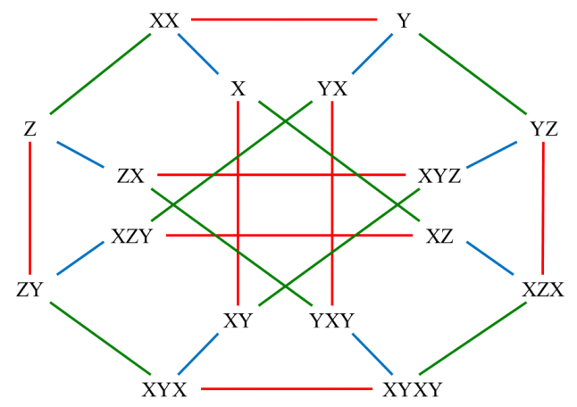
Generating the group using these generators, as illustrated in Generation of a Group, gives us a total of 16 elements: $$\begin{align}G_1=\{\,&X,\,Y,\,Z,\,XX,\,XY,\,XZ,\,YX,\,YZ,\,ZX,\,ZY,\\&XYX,\,XYZ,\,XZX,\,XZY,\,YXY,\,XYXY\,\}.\end{align}$$ The generation of the group can be illustrated using a Cayley graph:

The Cayley Graph for the Generated Pauli Group
Here, multiplication with \(X\), \(Y\) and \(Z\) are represented by a blue, red and green line respectively.

Note that all three generators \(X\), \(Y\) and \(Z\) are their own inverse. For example $$YY=\begin{bmatrix}0&-i\\i&0\end{bmatrix}\begin{bmatrix}0&-i\\i&0\end{bmatrix}=\begin{bmatrix}1&0\\0&1\end{bmatrix}=I.$$ This implies that all operations in the Cayley graph are symmetrical. We therefore use no arrows in the Cayley graph, and any edge can be used in both directions. As another consequence, the neutral element \(I\) is represented as \(XX\).

Each element of the group can be represented in many different ways. For example, it is easy to observe the following equations in the Cayley graph: $$XYZ=YZX=ZXY.$$ The generation process implicitly checks for equal matrices. The notation of the elements above is merely depending on the order in which the generators are combined. The first time a new matrix is obtained, it is added to the set, while subsequent occurrences of the same matrix will not be added to the set.

Enumerating the Pauli Group

The Pauli group can also be defined by enumeration of all elements, using the identity matrix and the generator matrices introduced earlier, multiplied by one of a number of complex factors: $$G_1=\{fA,f\in\{\pm 1,\pm i\},A\in\{I,X,Y,Z\}\}.$$ Consider the matrix multiplication $$XY=\begin{bmatrix}0&1\\1&0\end{bmatrix}\begin{bmatrix}0&-i\\i&0\end{bmatrix}=\begin{bmatrix}i&0\\0&-i\end{bmatrix}=iZ.$$ It is easy to verify that each element of the generated definiton of the group can be written as an element of the enumerated definition of the group. As such, the enumerated group is identical to the generated group. We intentionally do not use the term isomorphic, as the matrices in both groups are identical and the difference is merely in naming.

We can therefore rename the nodes in the Cayley graph based on this enumeration:

The Cayley Graph for the Enumerated Pauli Group

Alternative Generators

Using the Cayley graph, one can observe the symmetry of the generators, in the sense that an even permutation of the generators will not change the structure of the Cayley graph. An even permutation of \(X\), \(Y\) and \(Z\) still yields a correct Cayley graph, where the edges duly represent matrix multiplications. Odd permutations however would require some nodes to trade places in order for the group to be correctly represented.

Looking at the way the group is generated by the three generators, each combination of two generators will generate exactly half of the group. In fact, that is the case for any pair of independent elements of the group.

Applying the generators one after the other, alternatingly, enumerates half of the group in a loop. The third generator is required to get to the other half of the group, where the same loop structure occurs. In fact, that is the case for any combination of generators of the group.

We will now move on to an alternative construction of the Pauli group, as the central product of the cyclic group of order four and the dihedral group of a square.

The Cyclic Group of Order Four

The cyclic group of order 4 is a group with one generator that yields the identity after 4 applications. It can be defined as the additive group of integers modulo 4: $$C_4=\mathbb{Z}/4\mathbb{Z}=\{0,1,2,3\}.$$ Note that a number refers to the equivalence class of that number in the quotient group here.

As we can only represent finite groups, we cannot use the definition based on a quotient group of \(\mathbb{Z}\). We will be using the finite set of integers modulo 4 and define the addition operation on that set, as illustrated in Cyclic Groups.

The Cayley graph for the group is

The Cayley Graph for the Cyclic Group of Order 4
In what follows, we will need the center of \(C_4\). The center of a group is defined as the set of elements that commute with every element in the group. The center of a group \(G\) is denoted and defined by $$Z(G)=\{z\in G|\forall g\in G, zg=gz\}.$$ As \(C_4\) is an Abelian group, its center is the group itself: $$Z(C_4)=C_4=\{0,1,2,3\}.$$ Note that we could just as well create a cyclic group of order 4 using for example the matrix representation of a 90 degrees rotation as a generator. Borrowing on the notation of the Pauli matrices, that would be using the matrix $$R=XZ=\begin{bmatrix}0&1\\1&0\end{bmatrix}\begin{bmatrix}1&0\\0&-1\end{bmatrix}=\begin{bmatrix}0&-1\\1&0\end{bmatrix}.$$ The group would then be defined as the set $$C_4=\{I,R,R^2,R^3\},$$ with composition (matrix multiplication) as an operation.

Note that we could have used any combination of two generators of the Pauli group, in any order, as they will all cycle after four applications. Defining \(R\) as \(XZ\) is just an example with an intuitive meaning.

We could use the matrix representation of \(C_4\) to continue. However, we opted for the integers modulo 4, just to illustrate using groups with different types of elements in our constructions.

The Dihedral Group of a Square

A dihedral group is the symmetry group of a regular polygon. In this case, we need the dihedral group of a square, denoted \(D_8\) in abstract algebra, denoted \(D_4\) in geometry. The group can be generated using two generators: a rotation over 90 degrees, denoted R, and mirroring against the verical axis, denoted M.

We can represent those generators by matrices once more, as transformations in a plane: $$M=\begin{bmatrix}1&0\\0&-1\end{bmatrix},\,R=\begin{bmatrix}0&-1\\1&0\end{bmatrix}.$$ Generating the group using these generators, as illustrated in Generation of a Group, gives us a set of 8 elements: $$D_8=\{I,R,RR,RRR,M,RM,RRM,MR\}.$$ with composition (matrix multiplication) as an operation.

The Cayley graph for this group is

The Cayley Graph for the Dihedral Group of a Square
A red arrow represents multiplication by \(R\), a blue line represents multiplication by \(M\). As before, as \(M\) represents a symmetric operation, the arrows for that generator have been left out.

In what follows, we will need \(Z(D_8)\), the center of \(D_8\). As illustrated in The Center of a Group, we get $$Z(D_8)=\{I,RR\}.$$ That is, besides the identity, \(RR\) is the only element that commutes with every other element in the group.

Note that our center is isomorphic to the cyclic group of order 2: $$Z(D_8)\cong C_2.$$

The Central Product

On the Wikipedia page on the Pauli group, we read that the Pauli group is isomorphic to the central product of the cyclic group of order four and the dihedral group of a square: $$G_1\cong C_4\circ D_8.$$ As a reminder, the Wikipedia page on the central product states that the central product is similar to the direct product, but in the central product two isomorphic central subgroups of the smaller groups are merged into a single central subgroup of the product.

The Direct Product

The set of elements of the direct product of \(C_4\) and \(D_8\) is the cartesian product of the factor groups: $$C_4\times D_8 = \{(n, A)\,|\,n\in C_4, A\in D_8\}.$$ The operation for the direct product is the pairwise application of the operations of the factor groups. Assuming that \(+\) is the group operation of \(C_4\), being the additive group of integers modulo 4, matrix multiplication in \(D_8\) is denoted by juxtaposition, and \(\times\) is the group operation of the direct product, we get: $$(n, A)\times (m, B) = (n+m, AB).$$

The Common Center

Looking at the centers of \(C_4\) and \(D_8\), it is easy to see that the maximum subgroup they have in common is isomorphic to \(C_2\), the cyclic group of order 2. Formulated over the respective alphabets, we get $$\{0, 2\}\cong\{I, RR\}\cong C_2.$$ We will therefore express the commonality using the subgroup \(Z\) of the direct product isomorphic to the common center of the factor groups as: $$Z=\{(0, I), (2, RR)\}\cong C_2.$$ Clearly, \((0, I)\) is the neutral element of the direct product, and consequently also of \(Z\). We quickly verify the cyclic nature of \(Z\), for illustration: $$(2, RR)\times (2, RR) = (2+2, RRRR) = (0, I).$$

An Alternative Definition of the Pauli Group

Now, finally, we are ready to try constructing our alternative Pauli group, as a quotient group we will refer to as \(F_1\), dividing the direct product by the subgroup \(Z\): $$G_1\cong F_1=(C_4\times D_8)/Z.$$ Although we did use the notion of a quotient group already talking about the set of integers modulo 4, we quickly repeat the definiton of a quotient group as given on Wikipedia: $$G/N=\{gN\,|\,g\in G\},$$ where \(G\) is a group and \(N\) is a normal subgroup. Here, \(gN\) is referred to as a coset of \(N\) in \(G\). Typically, different elements \(g\) will result in the same coset when applied to \(N\).

However, for simplicity in notation, for the representation of the quotient group, we will use a representative of each coset rather than the coset iself. For example, we will use \((1, M)\) as the representative of its coset $$(1, M)\times Z=\{(1, M), (3, RRM)\}$$ As such, and as illustrated in The Central Product, we get the following enumeration for the quotient group: $$\begin{align}F_1=\{&(0,I), (0,R), (0,M), (0,RR), (0,RM), (0,MR), (0,RRR), (0,RRM),\\&(1,I), (1,R), (1,M), (1,RR), (1,RM), (1,MR), (1,RRR), (1,RRM)\}\end{align}$$ So far so good, but is this group \(F_1\) really isomorphic to the Pauli group ?

Finding the Isomorphism

To verify whether \(F_1\) is isomorphic to \(G_1\), we have to find a bijection \(\phi\) between the elements of both groups that preserves the group operation. That is, for \(A\) and \(B\) elements of \(G_1\): $$\phi(AB)=\phi(A)\times\phi(B).$$ First of all, the number of elements is fine: \(F_1\) has 16 elements, just as the Pauli group. However, the remainder of the exercise is a bit harder.

We can restrict ourselves to defining the bijection for the generators only, and then verifying preservation of the operation on all combinations (including repetitions) of the generators.

Candidate mappings for the generators should respect a number of constraints. First of all, the identity element can be excluded. Secondly, all generators should be their own inverse, as is the case for \(X\), \(Y\) and \(Z\). This reduces the candidate set to seven elements: $$\{(0,M), (0,RR), (0,RM), (0,MR), (0,RRM), (1,R), (1,RRR)\}$$ Furthermore, logic dictates that in our combination of three generators, all basic building blocks should be represented, in particular the elements \(0\), \(1\), \(R\) and \(M\) of the respective factor groups. This leaves \(2\times 4\times 5=40\) possible combinations of three, ignoring order.

In the java section on Finding an Isomorphism, we do an exhaustive scan, mapping \(X\), \(Y\) and \(Z\) onto different combinations of elements of \(F_1\). Here, we limit ourselves to presenting one of the resulting isomorphisms: $$\phi(X)=(0, M),\,\phi(Y)=(0, RM),\,\phi(Z)=(1, R).$$ Once we have the bijection defined for the generators, the entire group structure follows nicely. This is illustrated once again by a Cayley diagram, the equivalent of the ones presented earlier, but now over our new alphabet:

The Cayley Graph for the Central Product
Note that many more mappings are possible to define the isomorphism, given the symmetries of the Pauli group, and the one presented here represents just one possiblity.

Conclusions

We verified exhaustively that the Pauli group on a single qubit, typically defined as the group generated by three 2x2 matrices over the complex domain, is isomorphic to the central product of the cyclic group of order four and the dihedral group of a square. There's no magic involved here.

Java Implementation

However, the fun in this post is found in the way finite groups can be represented in Java, using whatever type of element and operation that suits the purpose. In addition, constructs such as the direct product, the center and the quotient of groups can be implemented generically on these groups. In what follows, we will illustrate this implementation in Java.

Group Representation

We start our implementation in Java with the definition of the interface that defines a group:

public interface Group<T> {

	public Set<T> getElements();
	public T getIdentity();
	public T multiply(T a, T b);

}

It is defined as a generic interface, where the element type is a parameter. We do not impose any explicit type for the elements of a group, merely that the element type implements equals and hashcode.

A group should be able to produce its elements, as a Java Set, it provides access to the neutral element, and it implements the group operation, referred to as mul.

Note that the group operation could be implemented on the element as well, but that would require an explicit element type, which strongly reduces the genericity of the group implementation.

Also note that we did not include the concepts of symmetric elements, as we do not need them in the scope of this post. We are confident that this could be added to the implementation without breaking the approach taken.

Enumeration of a Group

As a first implementation of the group interface we will focus on an enumerated group:

public class EnumeratedGroup<T> implements Group<T> {

    private Set<T> elements;
    private T identity;
    private BiFunction<T, T, T> operation;

    public EnumeratedGroup(Set<T> elements, T identity, BiFunction<T, T, T> operation) {
        this.elements = new HashSet<>(elements);
        this.identity = identity;
        this.operation = operation;
    }

    ...

    @Override
    public T multiply(T a, T b) {
        return operation.apply(a, b);
    }

}

The constructor of the group requires the set of elements of the group, an explicit reference to the identity element, and a binary function that implements the group operation.

The implementation of this class is straightforward now. You will want to add getters and at least provide an implementation for toString. We only included the implementation of the multiply function, just in case.

Generation of a Group

Next comes the implementation of a group specified using a finite set of generators:

public class GeneratedGroup<T> implements Group<T> {

    private Set<T> generators;
    private Set<T> elements;
    private T identity;
    private BiFunction<T, T, T> operation;

    public GeneratedGroup(Set<T> generators, T identity, BiFunction<T, T, T> operation) {
        this.generators = generators;
        this.identity = identity;
        this.operation = operation;
    }

    @Override
    public Set<T> getElements() {
        if (elements==null) {
            elements = new HashSet<>(generators);
            elements.add(getIdentity());
            int size = 0;
            while (size<elements.size()) {
                size = elements.size();
                Set<T> generated = new HashSet<>();
                for (T t : elements) {
                    for (T g : generators) {
                        generated.add(multiply(t, g));
                    }
                }
                elements.addAll(generated);
            }
        }
        return elements;
    }

    ...

}

Again, simple implementation details are left out.

The thing worth mentioning here is the getElements function, implemented lazily. On first invocation, it will generate the set of elements based on the identity element and the set of generators using a fixed point approach:

• We start with the set of elements consisting of the identity element only.
• We then keep applying all generators to all elements of this set, and adding these as new elements, until the set no longer grows in size.

The Pauli Group

We now have sufficient building blocks to implement a first version of the Pauli group, with matrices as elements, using generators. We will be using the matrices introduced in Generating the Pauli Group.

We will be borrowing the matrix implementation of our previous post about quantum computing, Hadamard and Friends. And we have an alphabet of matrices ready:

public class Alphabet {

    public static final Matrix I = MatrixUtils.identity(2);

    public static final Matrix X = new Matrix("X", new Double[][] { { 0d, 1d }, { 1d, 0d } });
    public static final Matrix Y = new Matrix("Y", new Double[][] { { 0d, -1d }, { 1d, 0d } }).cmul(Complex.I).setName("Y");
    public static final Matrix Z = new Matrix("Z", new Double[][] { { 1d, 0d }, { 0d, -1d } });

    ...

}

Multi-dimensional complex array constants are cumbersome to write, and the Matrix implemention is immutable. Therefore, we have to rename the matrix \(Y\) after multiplication with the complex number \(i\).

The Pauli group can now easily be defined as:

public class GroupUtils {

    public static Group<Matrix> getPauliGroup() {
        Set<Matrix> generators = new HashSet<>(Arrays.asList(Alphabet.X, Alphabet.Y, Alphabet.Z));
        return new GeneratedGroup<Matrix>(generators, Alphabet.I, (a, b) -> a.vmul(b));
    }

    ...

}

Cyclic Groups

For the alternative implementation of the pauli group, we first need a cyclic group of order four. We cannot define this group as the quotient \(\mathbb{Z}/4\mathbb{Z}\), as we can only handle finite groups. We will therefore explicitly define modulo numbers and once more use a generated group.

public class Modulo {

    private int value;
    private int modulo;

    public Modulo(int value, int mod) {
        this.value = value%mod;
        this.modulo = mod;
    }

    public Modulo add(Modulo m) {
        return new Modulo(value+m.getValue(), modulo);
    }

    ...

}

Completing the implementation is straightforward. We added the implementation of the group operation add, just in case.

The cyclic group of order four can now be easily defined as:

public class GroupUtils {

    public static Group<Modulo> getCyclicGroup(int size) {
        HashSet<Modulo> generators = new HashSet<>(Arrays.asList(new Modulo(1, size)));
        return new GeneratedGroup<Modulo>(generators, new Modulo(0, size), (a, b) -> a.add(b));
    }

    ...

}

The Dihedral Group of Order Eight

The dihedral group of order eight can equally be defined as a generated group, using the matrices introduced in The Dihedral Group of a Square. Therefore, this section is very similar to the one where we introduced the matrix representation of The Pauli Group.

First we need the matrix definitions:

public class Alphabet {

    public static final Matrix R = new Matrix("R", new Double[][] { { 0d, -1d }, { 1d, 0d } });
    public static final Matrix M = new Matrix("M", new Double[][] { { 1d, 0d }, { 0d, -1d } });

    ...

}

Then we are ready to create the group:

public class GroupUtils {

    public Group<Modulo> getDihedral8Group() {
        Set<Matrix> generators = new HashSet<>(Arrays.asList(Alphabet.R, Alphabet.M));
        return new GeneratedGroup<Matrix>(generators, Alphabet.I, (a, b) -> a.vmul(b));
    }

    ...

}

The Center of a Group

Comes the time we need to compute the center of a group:

public class GroupUtils {

    public static <T> Group<T> getCenter(Group<T> group) {
        Set<T> center = group.getElements().stream()
            .filter(z -> group.getElements().stream()
                .filter(g -> !group.multiply(z, g).equals(group.multiply(g, z))).count()==0l)
            .collect(Collectors.toSet());
        return new EnumeratedGroup<T>(center, group.getIdentity(), group::multiply);
    }

    ...

}

We provide a stream style implementation, that filters all elements of the group (the outer filter) that commute with all elements of the group (the inner filter) to determine the elements of the center. We then use that set to create an enumerated group with the same identity element and the same group operation.

The Direct Product

By now, the exercise risks becoming just more of the same thing. We can implement the direct product of two groups as the Cartesian product of the elements in the group with the pairwise group operations.

public class ProductGroup<T, S> implements Group<Pair<T, S>> {

    private Group<T> tgroup;
    private Group<S> sgroup;
    private Set<Pair<T, S>> elements;

    public ProductGroup(Group<T> tgroup, Group<S> sgroup) {
        this.tgroup = tgroup;
        this.sgroup = sgroup;
    }

    @Override
    public Set<Pair<T, S>> getElements() {
        if (elements==null) {
            elements = new HashSet<>();
            for (T t : tgroup.getElements()) {
                for (S s : sgroup.getElements()) {
                    elements.add(new Pair<>(t, s));
                }
            }
        }
        return elements;
    }

    @Override
    public Pair<T, S> getIdentity() {
        return new Pair<>(tgroup.getIdentity(), sgroup.getIdentity());
    }

    @Override
    public Pair<T, S> multiply(Pair<T, S> a, Pair<T, S> b) {
        return new Pair<>(tgroup.multiply(a.getT(), b.getT()), sgroup.multiply(a.getS(), b.getS()));
    }

    ...

}

We us a Pair to combine two elements, one of each group. You can use any implementation you can find, or write your own. Just make sure to implement equals and hashcode in a proper way.

Again we have a lazy implementation of the getElements method that calculates the Cartesian product of the elements of the two groups as a set of pairs. The identity element is the pair of the identity elements of both groups. The operation is the pairwise multiplication of the elements of both groups.

Quotient Groups

The implementation of a quotient group however is a bit trickier:

public class QuotientGroup<T> implements Group<T> {

    private Group<T> group;
    private Set<T> subgroup;
    private Set<T> elements;
    private Map<T, Set<T>> representation;

    public QuotientGroup(Group<T> group, Set<T> subgroup) {
        this.group = group;
        this.subgroup = subgroup;
    }

    @Override
    public Set<T> getElements() {
        if (elements==null) {
            elements = new HashSet<>();
            representation = new HashMap<>();
            Set<Set<T>> cosets = new HashSet<>();
            for (T e : group.getElements()) {
                Set<T> coset = GroupUtils.multiply(group, subgroup, e);
                if (!cosets.contains(coset)) {
                    elements.add(e);
                    representation.put(e, coset);
                    cosets.add(coset);
                }
            }
        }
        return elements;
    }

    @Override
    public T getIdentity() {
        return group.getIdentity();
    }

    private T normalize(T t) {
        T n = GroupUtils.findElement(representation, t);
        if (n!=null) {
            return n;
        }
        return t;
    }

    @Override
    public T multiply(T a, T b) {
        return normalize(group.multiply(a, b));
    }

    ...

}

We start with a group and a subgroup, the latter represented as a set of elements only. In addition to that, the impementation will keep track of the set of elements, as most of the Group implementations. However, as we will represent each coset by a unique representative of the coset, we need to keep track of which element represents which coset. This is done using the representation, a mapping of represtatives to cosets.

As before, the elements are determined lazily. To determine the set of elements, we scan the elements of the larger group and determine the coset of the smaller group for each element. Is this is a new coset, we use the element as a representative for that coset, and update the representation map. If we already have the coset, we replace the element by its representation.

The getElements function uses a utility function GroupUtils.multiply for this purpose, that determines the coset of an element of the group:

public class GroupUtils {

    public static <T> Set<T> multiply(Group<T> group, Set<T> elements, T element) {
        return elements.stream().map(e -> group.multiply(e, element)).collect(Collectors.toSet());
    }

    ...

}

The QuotientGroup implementation has a private member function normalize that does the same thing, replacing an element by its unique representative, that we use after every calculation. For now, that is only in the multiply function. It uses another utility function GroupUtils.findElement, that finds the coset in the representation map that contains a newly created element, and returns the representation of that coset:

public class GroupUtils {

     public static <T> T findElement(Map<T, Set<T>> map, T t) {
        for (T r : map.keySet()) {
            if (map.get(r).contains(t)) {
                return r;
            }
        }
        return null;
    }

    ...

}

The Central Product

We now have sufficient building blocks to implement the second version of the Pauli group, as the central product of the cyclic group of order four and the dihedral group of a square.

public class GroupUtils {

    public static <T> Group<Pair<Modulo, Matrix>> getCentralProductPauliGroup() {
        Group<Modulo> cyclic4 = getCyclicGroup(4);
        Group<Matrix> dihedral8 = getDihedral8Group();
        Group<Pair<Modulo, Matrix>> product = new ProductGroup<>(cyclic4, dihedral8);
        Set<Pair<Modulo, Matrix>> subgroup = getCentralProductPauliSubGroup();
        return new QuotientGroup<>(product, subgroup);
    }

    public static <T> Set<Pair<Modulo, Matrix>> getCentralProductPauliSubGroup() {
        Set<Pair<Modulo, Matrix>> subgroup = new HashSet<>();
        subgroup.add(new Pair<>(new Modulo(0, 4), Alphabet.I));
        subgroup.add(new Pair<>(new Modulo(2, 4), r.vmul(r)));
        return subgroup;
    }

    ...

}

Note that we explicitly construct the subgroup of the direct product isomorphic to the maximum common subgroups of the centers of both factor groups of the direct product. Let's say we leave the generic implementation of that step as an exercise.

Finding an Isomorphism

Verifying whether a mapping between groups is an isomorphism is easy. Assume we represent the isomorphism as a mapping of elements from one group to the other:

public class GroupUtils {

    public static <T, S> boolean isIsomorphism(Group<T> tgroup, Group<S> sgroup, Map<T, S> map) {
        if (tgroup.getElements().size()!=sgroup.getElements().size()) {
            return false;
        }
        for (T a : tgroup.getElements()) {
            for (T b : tgroup.getElements()) {
                if (!map.get(tgroup.multiply(a, b)).equals(sgroup.multiply(map.get(a), map.get(b)))) {
                    return false;
                }
            }
        }
        return true;
    }

    ...

}

If the number of elements in both groups is different, the groups cannot possibly be isomorphic. Otherwise, we just check any combination of two elements of the first group, and verify whether the product of the images of the elements equals the image of the product. Any mismatch will refute the isomorphic character of the mapping.

Finding an isomorphism between two groups is trickier. Suppose we have generators for both groups, then we can gradually construct the isomorphism, and check for inconsistencies along the way:

public class GroupUtils {

    public static <T, S> Map<T, S> getIsomorphism(Group<T> tgroup, Group<S> sgroup, List<T> tgenerators, List<S> sgenerators) {
        if (tgenerators.size()!=sgenerators.size()) {
            return null;
        }
        Map<T, S> isomorphism = new HashMap<>();
        isomorphism.put(tgroup.getIdentity(), sgroup.getIdentity());
        for (int i=0; i<tgenerators.size(); ++i) {
            isomorphism.put(tgenerators.get(i), sgenerators.get(i));
        }
        int size = 0;
        while (isomorphism.size()>size) {
            size = isomorphism.size();
            Map<T, S> mapping = new HashMap<>();
            for (T t1 : isomorphism.keySet()) {
                for (T t2 : isomorphism.keySet()) {
                    T tproduct = tgroup.multiply(t1, t2);
                    S sproduct = sgroup.multiply(isomorphism.get(t1), isomorphism.get(t2));
                    S expected = isomorphism.get(tproduct);
                    if (expected==null) {
                        expected = mapping.get(tproduct);
                    }
                    if (expected==null) {
                        mapping.put(tproduct, sproduct);
                    } else if (!sproduct.equals(expected)) {
                        return null;
                    }
                }
            }
            isomorphism.putAll(mapping);
        }
        return isomorphism;
    }

    ...

}

In what follows we will refer to the first group as the domain of the isomorphism and to the second group as the image of the isomorphism.

We assume that the list of generators that are provided for both groups already reflect the isomorphism. Therefore, they should be of equals size.

Then we initialize the isomorphism with the generators. We then extend the isomorphism by trying all combinations of elements in the domain, and calculating the products of their images and the image of their product. If the product is not yet present in the domain of the isomorphism, we add a mapping. If the product is present already, its image in the isomorphism should be equals to what we just calculated.

Because we cannot iterate over a collection while it is being modified, we accumulate new mappings in a separate data structure. We then merge all new mappings into the isomorphism after all combination of elements in the domain have been processed.

We repeat this process until the isomorphism no longer grows in size, effectively finding a fixed point for the process. Under the assumption that the initial elements provided are generators for the doamin and the image of the isomorphism, respectively, the fixed point will represent an isomorphism between both groups.

We realize this is all a bit messy, but we basically come to the same conclusion as Naftali Harris on this subject: finding an isomorphism between two groups is not a trivial task. However, using generators will reduce the complexity in a significant way.

Selecting Generators

The only step remaining to close the loop here, is finding the generators for the image. We will leave out the coding details, but give you the results.

We already have the generators for the domain, being \(X\), \(Y\) and \(Z\). Starting with all 16 elements of the image, we can limit ourselves to those that are a root of the identity element, as we know this condition holds for the generators of the domain. Excluding the identity itself, we find 7 elements that square to the identity:

[(0,M), (0,RR), (0,RM), (0,MR), (0,RRM), (1,R), (1,RRR)]

If we try each combination of three elements out of this set, no repetition, order matters, we get \(7!/3!=210\) possible combinations. Out of these, it turns out that \(48\) can be used to construct an isomorphism.

Knowing that the group structure is invariant under permutations of those three generators, and there are \(3!=6\) permutations of three elements, we get \(48/6=8\) combinations, ignoring order, that do the job. Here they are:

[
  [(0,M), (0,RM), (1,R)], [(0,M), (0,RM), (1,RRR)],
  [(0,M), (0,MR), (1,R)], [(0,M), (0,MR), (1,RRR)],
  [(0,RM), (0,RRM), (1,R)], [(0,RM), (0,RRM), (1,RRR)],
  [(0,MR), (0,RRM), (1,R)], [(0,MR), (0,RRM), (1,RRR)]
]

Conclusions

Wrapping the standard Java Set interface and its implementations with some additional characteristics provides an easy way to implement finite groups and play around with them. As can be expected however, one quickly gets into the realms of NP-complete problems. For the Pauli group on a single qubit, the limited quantitative complexity helped us to gain some insights.

Hadamard and Friends

Playing around with Quantum Computing - Getting familiar with quantum bits, gates, wires and circuits, and the algebra behind them - Trying brute force search on quantum circuit space.

Introduction

Latent interest in the subject of quantum computing was awoken during an evening lecture by IBM. After reading Quantum computing for the very curious, we decided to take on the subject. The initial objective was to search quantum circuit space to find a circuit that implements the Toffoli gate.

A Quantum Circuit for the Toffoli Gate
Let's be clear about it: we did not meet that objective. Quantum circuit space is way too vast to be explored using classical computing by brute force alone. Hence the hype. And we were missing the knowledge and intuition to compensate for that fact using heuristics or other shortcuts.

However, we did learn how to create the matrix representation of a quantum circuit. That is the essence of this post, on which the brute force search is based. The section Matrix Representations provides a formal summary.

In addition, the brute force technique developed helped us in gaining insight and making interesting observations in the domain. And we were able to find a quantum circuit for some simpler problems, such as controlled Pauli gates and the simplest quantum Fourier transform.

Information Sources

We will provide references wherever we feel they are relevant. However, introductions that we found useful include:

• Quantum computing for the very curious, as said before, the main trigger for this exercise, and a detailed introduction to the subject. Beware, a first reading will take a couple of hours to complete. Also, the article does not focus too much on the matrix representation that is the main focus of this post.
• A field guide to quantum computing, by IBM, an excellent introduction to the subject. It covers the subject with more speed, and consequently takes you a lot further. The material is accompanied by OpenQasm and Qiskit examples, to try things out. Note however that we will not be using any of these in the context of this post.
• Wikipedia's page on quantum logic gates and many other Wikipedia pages related to quantum computing. The information on the pages is of high quality, and after reading the former sources, can be digested without too many obstacles.

Before we start, we wish to thank the Belgian IBM staff explicitly for organising evening lectures on the status of IBM's developments in quantum computing. They are very instructive, and actually preceded all our other reading in the domain.

Prerequisites

If you are not familiar with quantum computing and the concepts and notations of the domain, we invite you to at least skim one of the sites mentioned under Information Sources first.

We encourage you not to be scared off by the rather mathematical notation, as the basic concepts remain fairly simple. If you are familiar with complex numbers and have a basic knowledge of matrices, you should be fine.

Matrix Representations

We provide a formal overview of how to create the matrix representation of a quantum circuit and its parts here. We will make a strict distinction between quantum entities and their matrix representations, and use \({\oldstyle M}(...)\) to denote the matrix representation of any quantum entity, including quantum states, gates, circuits and circuit layers.

In practice, some quantum entities and their matrix representations are often denoted using the same symbol. With the exception of this section, we will also take that liberty throughout this post.

Computational basis states of a qubit: The computational basis states of a single qubit are represented by 2x1 matrices, vectors. $${\oldstyle M}(|0\rangle)=\begin{bmatrix}1\\0\end{bmatrix}, {\oldstyle M}(|1\rangle)=\begin{bmatrix}0\\1\end{bmatrix}$$ Here, \(|0\rangle\) and \(|1\rangle\) are the computational basis states of a single qubit.

The quantum state of a qubit: The quantum state of a qubit is expressed as a linear combination of the computational basis vectors with complex coefficients and length 1, represented as a vector with the coefficients of that linear combination. $${\oldstyle M}(|\psi\rangle)={\oldstyle M}(\alpha|0\rangle+\beta|1\rangle)=\begin{bmatrix}\alpha\\\beta\end{bmatrix}$$ Here, \(|\psi\rangle\) is the quantum state of a single qubit.

Computational basis states of a collection of qubits: The computational basis states of a collection of qubits are represented by 2\(^N\)x1 matrices, vectors, defined as the tensor product of the computational basis state representation for each qubit in the collection. $${\oldstyle M}(|q_1q_2...q_N\rangle)={\oldstyle M}(|q_1\rangle)\otimes{\oldstyle M}(|q_2\rangle)...{\oldstyle M}(|q_N\rangle)$$ Here, \(|q_i\rangle, i=1...N\) represent computational basis states of the individual qubits. That is, \(q_i, i=1...N\) equal 0 or 1.

The quantum state of a collection of qubits: The quantum state of a collection of qubits is expressed as a linear combination of the computational basis vectors with complex coefficients and length 1, represented as a vector with the coefficients of that linear combination. It can be written as the tensor product of the vectors representing the quantum state of the individual qubits. $${\oldstyle M}(|\psi_1\psi_2...\psi_N\rangle)={\oldstyle M}(|\psi_1\rangle)\otimes{\oldstyle M}(|\psi_2\rangle)...{\oldstyle M}(|\psi_N\rangle)$$ Here, \(|\psi_1\psi_2...\psi_N\rangle\) represents the quantum state of the collection of qubits and \(|\psi_i\rangle, i=1...N\) represent the quantum states of the individual qubits.

You will not be using this rule very often. You will typically start with one of the computational basis states and then travel through a quantum circuit using the rules below.

Single wire quantum gates: Any single wire quantum gate operating on a single qubit can be represented by a unitary 2x2 matrix with complex elements. All quantum operations must be linear, so it suffices to describe the function on each one of the basis states and let the mixed states be defined by linearity. $${\oldstyle M}(G|0\rangle)=\begin{bmatrix}\alpha\\\beta\end{bmatrix},{\oldstyle M}(G|1\rangle)=\begin{bmatrix}\gamma\\\delta\end{bmatrix} \Rightarrow {\oldstyle M}(G)=\begin{bmatrix}\alpha&\gamma\\\beta&\delta\end{bmatrix}$$ Here, \(G\) represents a quantum gate, and we use juxtaposition to indicate the application of a gate to a qubit's quantum state.

Single wire quantum gate application: The matrix product is used for the application of a single wire gate to a qubit's quantum state. $${\oldstyle M}(G|\psi\rangle)={\oldstyle M}(G){\oldstyle M}(|\psi\rangle)$$ A series of single wire gates: To apply multiple gates to a qubit, multiply the matrix representation of the gates in reverse order. $${\oldstyle M}(G_1 G_2 ... G_N)={\oldstyle M}(G_N)...{\oldstyle M}(G_2){\oldstyle M}(G_1)$$ Here, \(G_i, i=1...N\) represent gates, and we use juxtaposition to indicate the serial application of multiple gates to the quantum state of a single qubit.

Strictly speaking, this rule is redundant, as it is a special case for a quantum circuit with only one wire, and as such it is covered by the more generic matrix representation rules following below. In any case, it should not be used when deriving the matrix representation of a quantum circuit with multiple wires.

Parallel single wire gates, layers: To apply a collection of gates to a collection of qubits in parallel, apply the tensor product to the matrices of the gates, in order. $${\oldstyle M}(G_1\parallel G_2...G_N)={\oldstyle M}(G_1)\otimes{\oldstyle M}(G_2)...{\oldstyle M}(G_N)$$ Here, we use the \(\parallel\) operator to indicate the parallel application of multiple single wire gates to a collection of qubits. More precisely, the expression \(G_1\parallel G_2...G_N\) represents a layer in a quantum circuit consisting of \(N\) wires, each wire with its own gate.

The notation with the \(\parallel\) operator is not part of the general notational conventions in quantum computing. However, we need a notation for a layer in a quantum circuit, because it is an intermediate level to determine the matrix representation of a quantum circuit. Hey, quantum computing is all about entanglement, and that's happening between different wires.

Whenever no gate is present in the layer on a wire \(i\), use the identity matrix \(G_i=I\).

Layer application: The matrix product is used for the application of a layer to the quantum state of a collection of qubits. $${\oldstyle M}(L|\psi_1\psi_2...\psi_N\rangle)={\oldstyle M}(L){\oldstyle M}(|\psi_1\psi_2...\psi_N\rangle)$$ Here, \(|\psi_1\psi_2...\psi_N\rangle\) represents the quantum state of the collection of qubits.

A series of layers, quantum circuits: To apply multiple layers to a collection of qubits, multiply the matrix representation of the layers in reverse order. $${\oldstyle M}(L_1 L_2...L_N)={\oldstyle M}(L_N)...{\oldstyle M}(L_2){\oldstyle M}(L_1)$$ Here, \(L_i, i=1...N\) represent layers, and we use juxtaposition to indicate the serial application of multiple layers in a quantum circuit.

Controlled gate, two wires: The matrix for a 2-wire layer consisting of a control gate and a controlled gate is the sum of two tensor products, one for the case where the control qubit state is \(|0\rangle\), and one for the case where the control qubit state is \(|1\rangle\). $${\oldstyle M}(C\parallel C(G))=P_0\otimes I+P_1\otimes{\oldstyle M}(G)$$ Here, \(C\) refers to the control gate and \(C(G)\) refers to the controlled gate \(G\), which is, for clarity, not restricted to the not gate \(X\). The matrices \(P_0\) and \(P_1\) realise the selection on the state of the control qubit and are defined as $$P_0=|0\rangle\langle 0|=\begin{bmatrix}1&0\\0&0\end{bmatrix}, P_1=|1\rangle\langle 1|=\begin{bmatrix}0&0\\0&1\end{bmatrix}.$$ The term control gate is not part of the general terminology in quantum computing, where the correct terms are a (2-wire) controlled gate with a control wire and a target wire. However, splitting the 2-wire controlled gate into two connected single wire entities greatly simplifies notation and implementation. We will refer to them as pseudo-gates.

Controlled gate, more than two wires: The matrix for a layer with more than two wires, containing a single control gate and a corresponding controlled gate, equally is the sum of two tensor products, one for the case where the control qubit state is \(|0\rangle\), and one for the case where the control qubit state is \(|1\rangle\), but in this case the products involve the matrix representations of the gates on other wires. $$ \begin{align} {\oldstyle M}(G_1&\parallel G_2...C_P...C(G_Q)...G_N)=\\ &{\oldstyle M}(G_1)\otimes{\oldstyle M}(G_2)...P_{0,P}...I_Q...{\oldstyle M}(G_N)+\\ &{\oldstyle M}(G_1)\otimes{\oldstyle M}(G_2)...P_{1,P}...G_Q...{\oldstyle M}(G_N) \end{align} $$ Here, \(P,Q=1...N\) with \(P\ne Q\). Furthermore, \(C_P\) means the control gate is on wire \(P\) and \(C(G_Q)\) means the controlled gate is \(G_Q\) on wire \(Q\). Also, \(P_{D,P},D=0,1\) is \(P_D\) in position \(P\) and \(I_Q\) is just the identity matrix in position \(Q\). And it should be clear that \(P\gt Q\) is allowed as well.

Multiple control wires: We did not investigate layers that contain a controlled gate with multiple control wires or multiple controlled gates working independently, but we expect a term is required in the sum of tensor products for all possible combinations of \(P_0\) and \(P_1\) for the different control gates, each term with the appropriate substitute matrix for the corresponding controlled gates.

Multi-wire gates, other than controlled: Also, the matrix representation rules should be extended to support multi-wire gates that are not control gates, such as the swap gate.

Brute Force Search on Quantum Circuit Space

With the rules for the matrix representation of quantum entities at hand, it is fairly simple to implement an abstract data type for a quantum circuit and simulate the quantum circuit. It comes down to the top-down derivation of the matrix representation of the underlying quantum elements and multiplying the matrix for the quantum circuit with the vector representation of the input for the circuit. Java code snippets are available at the end of this post, under the section Simulating a Quantum Circuit.

Note that the quantum state of a qubit is not directly observable. Suppose the quantum state of a qubit is given by $$|\psi\rangle=\alpha|0\rangle+\beta|1\rangle.$$ If that qubit is measured (in the standard basis), the result represented by \(|0\rangle\) is obtained with probability \(|\alpha|^2\) and the result represented by \(|1\rangle\) is obtained with probability \(|\beta|^2\), as prescribed by the Born rule. Therefore, strictly speaking, we do not simulate the quantum circuit. We merely calculate the probability amplitudes of the computational basis for the output of the quantum circuit.

Brute force search on quantum circuit space is then about finding a way to iterate over all possible quantum circuits, preferably in increasing order of complexity, and checking whether one of them implements the logic desired. Mission accomplished.

Surely this is not possible, as even quantum gates on itself already form an uncountable set. We will therefore restrict the quantum circuit space to a limited (finite) number of quantum gates, an alphabet say, on a case by case basis.

Brute Force Search on a Slice of Quantum Circuit Space

A little experimentation results in a fairly simple way to approach brute force search in this reduced context:

1. Fix the number of wires to be used for the quantum circuit.
2. Fix the "alphabet" of quantum gates to be used in the quantum circuit.
3. Fix the maximum number of layers part of the quantum circuit.
4. Generate all possible gate combinations for a single layer, using the gate alphabet and the number of wires.
5. Scan all possible quantum circuits by trying all combinations of these layers, starting with quantum circuits consisting of a single layer, and incrementally moving up to quantum circuits consisting of the maximum number of layers.

In this context, we only need a few simple building blocks, including the generation of the layers that can be created over the alphabet, the scanning of all quantum circuits that consist of a number of these layers, with a fixed maximum number of layers, an derivation of the matrix representation of such a quantum circuit, and a check function that determines whether a specific quantum circuit is the one we are looking for.

To keep circuit composition simple, and as briefly mentioned before, we will represent controlled gates by a pair of single wire pseudo-gates: a generic control gate on the control wire and a wrapper for the controlled gate on the controlled wire. This simplifies the layer generation, but may yield invalid configurations, for example with only a control gate or multiple controlled gates. To resolve this, we will filter out invalid layers after generation.

As can be expected by now, Java code snippets are available at the end of this post, under the section An Implementation of Brute Force Search.

In what follows, we will provide a number of examples where we scan quantum circuit space for a circuit implementing a specific logic, using this brute force search implementation.

Wolfgang Pauli

As a first example of the brute force search technique, we will have a closer look at a collection of three gates defined by the matrices: $$X=\begin{bmatrix}0&1\\1&0\end{bmatrix},Y=\begin{bmatrix}0&-i\\i&0\end{bmatrix}, Z=\begin{bmatrix}1&0\\0&-1\end{bmatrix}.$$ Here, \(X\) is the famous not gate.

These matrices are referred to as the Pauli matrices. They form a group of 16 elements, referred to as the Pauli group, that can be defined as $$G_1=\{fA,f\in\{\pm 1,\pm i\},A\in\{I,X,Y,Z\}\}$$ The Pauli group is generated by the elements \(X\), \(Y\) and \(Z\). The generation of the Pauli group based on these elements can be visualised using a Cayley graph:

A Cayley Graph for the Pauli Group
Here, blue lines indicate right multiplication with \(X\), red lines indicate right multiplication with \(Y\) and green lines indicate right multiplication with \(Z\). As all three of the generators are their own inverse, the connections are bidirectional.

Note that all three generators are required to cover the entire group. Leaving one generator out covers only half of the group.

On the Cayley graph, you can easily see for example that \(XZ=-iY\). This can be verified using the brute force technique, with the Pauli gates as an alphabet, a matrix equality check with the matrix \(-iY\) and a maximum of 2 layers. The search finds the quantum circuit:

A Quantum Circuit for \(-iY\)
We verify the matrix multiplication by hand, just this one time $$XZ=\begin{bmatrix}0&1\\1&0\end{bmatrix}\begin{bmatrix}1&0\\0&-1\end{bmatrix}=\begin{bmatrix}0&-1\\1&0\end{bmatrix}=-iY$$ Remember, for a series of single wire gates, the order of the gates is reversed for the matrix multiplication.

The hardest element of the Pauli group to generate with generators \(X\), \(Y\) and \(Z\), in terms of the number of operations, is \(-I\). We execute a brute force search, again with the Pauli gates as an alphabet, a matrix equality check with the matrix \(-I\), and a maximum of 4 layers. The search finds six quantum circuits, one of which is:

A Quantum Circuit for \(-I\)
The other quantum circuits found, written in gate order, not matrix order, are \(XZXZ\), \(YXYX\), \(YZYZ\), \(ZXZX\) and \(ZYZY\). It is easy to verify on the Cayley graph that these are all the shortest paths to derive \(-I\), starting at \(I\), with length 4.

Jacques Hadamard

Extending on the reach of the Pauli gates is the Hadamard gate, represented as $$H=\frac{1}{\sqrt{2}}\begin{bmatrix}1&1\\1&-1\end{bmatrix}.$$ Using the alphabet of the Pauli gates, extended with the Hadamard gate, we will use brute force search to find the inverse of the Hadamard gate.

In order to achieve this with our scanner, we create a checker that takes a matrix and checks whether the output of a circuit is the inverse of that matrix, by multiplying both and comparing the result with \(I\).

Brute force search for the inverse of \(H\) with a maximum of 1 layer yields

A Quantum Circuit for \(H^{-1}\)
This should not surprise us, as all quantum gates are represented by a unitary matrix, in particular the Hadamard gate, such that $$HH^\dagger=I.$$ And as \(H\) is its own conjugate transpose, it is also its own inverse.

We invite you to have a quick look at the Hadamard transform, to understand where the gate got its name.

Georges Remi

We will once more extend our reach and introduce the \(T\) gate and its conjugate transpose. These gates are defined as \(\pi/4\) rotations around the \(Z\) axis of the Bloch sphere: $$T=\begin{bmatrix}1&0\\0&e^{\frac{i\pi}{4}}\end{bmatrix}, T^\dagger=\begin{bmatrix}1&0\\0&e^{-\frac{i\pi}{4}}\end{bmatrix}.$$ We also introduce the phase gate \(S\), defined as a \(\pi/2\) rotation around the \(Z\) axis: $$S=\begin{bmatrix}1&0\\0&i\end{bmatrix}.$$ Clearly, given these definitions, \(S=TT\). But what's the inverse of S ?

Using the alphabet of all quantum gates that have been introduced so far, extended with \(T\), \(T^\dagger\) and \(S\), brute force search to find \(S^{-1}\), with a maximum of 2 layers yields

A Quantum Circuit for \(S^{-1}\)
Besides this circuit, other solutions found are \(SZ\) and \(ZS\). Check it out.

Daniel Gottesman and William Clifford

Another interesting collection of gates is the Clifford group. In Maris Ozols' paper on the Clifford group, we read that the group is generated by \(H\) and \(S\), the latter referred to as \(P\) in the paper.

We would love to present a Cayley diagram for the Clifford group, at least the one for 2x2 matrices. However, strictly speaking the group is defined as the unitaries that normailze the Pauli group, or as a quotient group, so that will require some extra work. For now, we note that we can generate 192 different 2x2 matrices using \(H\) and \(S\) as generators.

The Pauli gates can be expressed in function of the generators of the Clifford group. So let's try that, generating \(X\), \(Y\) and \(Z\) using \(H\) and \(S\) as generators.

A brute force search over the alphabet \(H\) and \(S\), a matrix equality check with the matrix for \(Z\) and a maximum of 2 layers finds

A Quantum Circuit for \(Z\)
A brute force search over the same alphabet, checking for the matrix for \(X\) requires 4 layers to find

A Quantum Circuit for \(X\)
Finally, checking for the matrix for \(Y\), we need 8 layers to find

A Quantum Circuit for \(Y\)

John Bell

The Bell states are states of two qubits with maximal entanglement. The concept of the Bell states has been used by John Bell in 1964 to prove that the result of some quantum mechanical experiments cannot be explained by a theory of local hidden variables, although the premise of statistical independence leaves room for alternative views, as argued by superdeterminism.

We will refer to a quantum circuit that can produce the Bell states out of the computational basis states as a Bell circuit. And we denote that circuit using \(B\).

We will try to find a Bell circuit using brute force search, using the same alphabet as before. The checker will apply the quantum circuit to the first computational basis state for two qubits and verify that the output is the first Bell state: $$B|00\rangle=\frac{|00\rangle+|11\rangle}{\sqrt{2}}.$$ A search limited to two layers finds

A Bell Circuit
The search also finds

Another Bell Circuit
As an illustration of the matrix representation rules, we will go through the trouble of verifying the first circuit in terms of matrix calculus and verify the circuit logic. The rules stipulate $${\oldstyle M}(B)={\oldstyle M}(C\parallel C(X)){\oldstyle M}(H\parallel I)=(P_0\otimes I+P_1\otimes X)(H\otimes I)$$ For the first layer, we have $$ H\otimes I=\frac{1}{\sqrt{2}}\begin{bmatrix}1&1\\1&-1\end{bmatrix}\otimes\begin{bmatrix}1&0\\0&1\end{bmatrix} =\frac{1}{\sqrt{2}}\begin{bmatrix}1&0&1&0\\0&1&0&1\\1&0&-1&0\\0&1&0&-1\end{bmatrix}. $$ For the second layer, we get the well known matrix for the controlled \(X\) gate $$ \begin{align} P_0\otimes I+P_1\otimes X &=\begin{bmatrix}1&0\\0&0\end{bmatrix}\otimes\begin{bmatrix}1&0\\0&1\end{bmatrix}+\begin{bmatrix}0&0\\0&1\end{bmatrix}\otimes\begin{bmatrix}0&1\\1&0\end{bmatrix}\\ &=\begin{bmatrix}1&0&0&0\\0&1&0&0\\0&0&0&0\\0&0&0&0\end{bmatrix}+\begin{bmatrix}0&0&0&0\\0&0&0&0\\0&0&0&1\\0&0&1&0\end{bmatrix} =\begin{bmatrix}1&0&0&0\\0&1&0&0\\0&0&0&1\\0&0&1&0\end{bmatrix}. \end{align} $$ And the multiplication of both is $$ {\oldstyle M}(B) =\begin{bmatrix}1&0&0&0\\0&1&0&0\\0&0&0&1\\0&0&1&0\end{bmatrix}\frac{1}{\sqrt{2}}\begin{bmatrix}1&0&1&0\\0&1&0&1\\1&0&-1&0\\0&1&0&-1\end{bmatrix} =\frac{1}{\sqrt{2}}\begin{bmatrix}1&0&1&0\\0&1&0&1\\0&1&0&-1\\1&0&-1&0\end{bmatrix}. $$ So finally we can verify the application of the circuit matrix to the first computational basis state as $$ {\oldstyle M}(B){\oldstyle M}(|00\rangle) ={\oldstyle M}(B)\begin{bmatrix}1\\0\\0\\0\end{bmatrix} =\frac{1}{\sqrt{2}}\begin{bmatrix}1\\0\\0\\1\end{bmatrix} =\frac{|00\rangle+|11\rangle}{\sqrt{2}}. $$

Daniel Greenberger, Michael Horne and Anton Zeilinger

We now continue our exercise by looking for the quantum states with maximal entanglement of three qubits. These are known as (the simplest case of) the Greenberger-Horne-Zeilinger (GHZ) states.

Using the same technique as for the first Bell state, we will search for a circuit \(C\) of 3 wires, that when applied to the first computational basis state, results in maximal entanglement: $$C|000\rangle=\frac{1}{\sqrt{2}}(|000\rangle+|111\rangle).$$ We get our first result when searching for a 3 layer circuit:

A GHZ Circuit
Searching for a circuit with 4 layers, another solution shows up:

Another GHZ Circuit
Looking at the Bell circuit and the GHZ circuit, you see the Hadamard gate introduces superposition and the controlled not gate introduces entanglement.

Felix Bloch

On wikipedia, we read that the controlled X gate seems to work like a classical gate in the computational basis \({|0\rangle,|1\rangle}\), but that things are different in the Hadamard tranformed basis \({|+\rangle,|-\rangle}\). Viewed in this basis, the state of the second qubit remains unchanged, and the state of the first qubit is flipped, according to the state of the second bit.

We invite you to try visualising this on this Bloch sphere.

Let's try to reproduce this by searching for alternative circuits for the controlled X gate. This can be done using the matrix checker, with the matrix of the controlled X gate we've seen before: $${\oldstyle M}(C\parallel C(X))=P_0\otimes I+P_1\otimes X.$$ Because the controlled X gate is in our alphabet (in the form of two single wire pseudo-gates \(C\) and \(C(X)\)), a myriad of trivial solutions appear. However, our targetted circuit is spawned as well:

A Controlled \(X\) in an Transformed Basis Circuit
Following the same path, we search for a circuit implementing the controlled \(Z\) gate, with matrix: $${\oldstyle M}(C\parallel C(Z))=P_0\otimes I+P_1\otimes Z.$$ Limiting the search to 3 layers yields 6 circuits, one of which is

A Controlled \(Z\) Circuit
Once more, we search for a circuit implementing the controlled \(Y\) gate, with matrix: $${\oldstyle M}(C\parallel C(Y))=P_0\otimes I+P_1\otimes Y.$$ Limiting the search to 4 layers this time yields 65 circuits, one of which is

A Controlled \(Y\) Circuit
and another one of which is

Another Controlled \(Y\) Circuit
You get a feeling of why \(T\) is a convenient gate in quantum circuit assembly.

Don Coppersmith

To continue, we will introduce the phase gates $$R_N=\begin{bmatrix}1&0\\0&e^\frac{2\pi i}{2^N}\end{bmatrix}.$$ Note that the phase gates are a generalisation of gates we introduced earlier, as \(S=R_2\) and \(T=R_3\).

We will now try to find a circuit for the Quantum Fourier transform (QFT) with 3 wires, which was invented by Don Coppersmith.

On the same Wikipedia page, from the QFT Example, we learn that the matrix for that circuit is referred to as \(F_8\), where $$F_8=\begin{bmatrix}\omega^{rc}, r,c=0...7\end{bmatrix},\omega=e^{\frac{\pi i}{4}}.$$ We execute a brute force search, this time with the alphabet reduced to \(I\), \(H\), the control pseudo-gate \(C\), the controlled phase gate of order 2 \(C(R_2)\) and the controlled phase gate or order 3 \(C(R_3)\). Using the matrix checker with \(F_8\), and limiting the search to 6 layers yields 32 circuits, one of which is

A QFT Circuit for 3 Wires
Obviously, playing with the minimal selection of gates can only be done because the circuit we are looking for is known beforehand. However, with an alphabet limited to 5 gates and 3 wires we have 125 possible layer configurations, which reduces after filtering for invalid combinations of the pseudo-gates to 32 layer configurations. Scanning circuit space for a circuit with 6 of these layers implies looking at over 1 billion circuits. More on that in the next section.

Tommaso Toffoli

We've finally come to our original objective: using brute force search on quantum circuit space to find a circuit for the Toffoli gate.

The Toffoli gate is a doubly controlled not gate, flipping the quantum state of the third wire only if the first two wires have quantum state \(|1\rangle\). It is represented by

The Toffoli Gate
The Toffoli gate is universal in classical reversible computing, in the sense that it can be used to implement any boolean function on a number of bits. In quantum computing however, that is not the case. But being able to implement the Toffoli gate using a quantum circuit implies that quantum computers are able to compute anything classical computers can compute.

A quantum circuit that implements the Toffoli gate is

A Quantum Circuit for the Toffoli Gate
Clearly, our objective to find a circuit for the Toffoli gate using brute force search on quantum circuit space was formulated heavily underestimating the combinatorial complexity of quantum circuit space.

Using the same reasoning as before, with an alphabet limited to 6 gates and 3 wires we have 216 possible layer configurations, which reduces after filtering for invalid combinations of the pseudo-gates to 32 (yes, 32 again) layer configurations. Scanning circuit space for a circuit with 12 of these layers implies looking at over 1 quintillion (10^18, or 1 billion billion) circuits. And that's knowing the minimal alphabet we have to use, because we already know the solution.

I guess we'll need a quantum computer to do that.

Conclusions

Our objective of scanning quantum circuit space for circuits that implement a specific logic has been extremely useful in getting familiar with the domain of quantum computing.

Reformulating all aspects of quantum circuit simulation to use the matrix representation of quantum entities and matrix operations gave us a uniform computational framework and was able to support our entire exercise.

And we got to know a lot of smart people.

As for finding a circuit for the Toffoli gate, we were beaten by the numbers. We did stumble upon a number of pathways to overcome the combinatorial complexity, and approach the problem using divide and conquer. However, that will require some more study and experimentation. Maybe in a future blog post ...

Java Implementation

For our implementation of the brute force search, written in Java (version 8), we need a limited number of building blocks: a library for matrix representation and manipulation over the complex domain, an abstract data type for the representation and simulation of quantum circuits, and finally an implementation of the brute force process.

We will provide representative code snippets for each of those building blocks in the next sections.

A Matrix Library over the Complex Domain

Matrix libraries in Java are plentiful. Even if you require matrices over the domain of the complex numbers, there are still a number of good options.

However, as we only need a limited set op basic operations on complex numbers and matrices over complex numbers, we took the matrix development into scope of the exercise. We will not elaborate on that implementation here, as this is a marginal topic for this post. We will limit ourselves to stating that the implementation features immutable classes Complex and Matrix, as well as a class MatrixUtils that provides some matrix utility functions.

You will find references to the matrix operations in the code snippets in the next sections. We assume class and function naming to be self-explaining.

Simulating a Quantum Circuit

The simulation of a quantum circuit starts with an abstract data type for the representation of quantum circuits.

The first quantum entity we will model is the quantum gate. The Gate interface specifies that a quantum gate is represented by a symbol and has an associated matrix.

public interface Gate {

    public String getSymbol();
    public Matrix getMatrix();
	
}

Commonalities between all gate implementations will be grouped in a base class NamedGate.

public class NamedGate implements Gate {

    private String symbol;
    private Matrix matrix;

    public NamedGate(String symbol, Matrix matrix) {
        this.symbol = symbol;
        this.matrix = matrix;
    }

    ...

}

The identity gate, which was omnipresent behind the screens, is implemented by the class IdentityGate as an extension of NamedGate.

public class IdentityGate extends NamedGate {

    public static final Matrix I = MatrixUtils.getIdentity(2);

    public IdentityGate() {
        super("I", I);
    }

}

It uses MatrixUtils::getIdentity to create a 2x2 identity matrix. Note that it keeps a static final reference to the identity matrix. Sharing the matrix of the identity gate over all instances can be done because the matrix data type is immutable.

The implementation of the Hadamard gate provides another example.

public class HadamardGate extends NamedGate {

    public static final Matrix H = new Matrix(new Double[][] { { 1d, 1d }, { 1d, -1d } }).smul(1d/Math.sqrt(2d));

    public HadamardGate() {
        super("H", H);
    }

}

This time, the matrix is created inline, again using a static final reference. Note that the Matrix::smul function implements the multiplication of a matrix with a scalar (Double) value.

As explained before, control gates are not implemented as 2-wire gates, but rather as a combination of two single wire pseudo-gates. The ControlGate class implements the part on the control wire.

public class ControlGate extends NamedGate {

    public ControlGate() {
        super("C", null);
    }

}

It merely acts as a placeholder, as you will see below.

The pseudo-gate for the target wire is implemented by the ControlledGate class, which acts as a wrapper for the controlled gate and in itself also implements the Gate interface.

public class ControlledGate extends NamedGate {

    private Gate gate;

    public ControlledGate(Gate gate) {
        super("C("+gate.getSymbol()+")", gate.getMatrix());
        this.gate = gate;
    }

    ...

}

You will see these pseudo-gates in action in a moment.

Next comes the implementation of a layer of a quantum circuit. We opted for the representation of a circuit as a sequence of layers, rather than a sequence of wires, which might seem more natural. However, as explained in the section Matrix Representations, the matrix representing a quantum circuit is not constructed out of wire matrices, but rather out of layer matrices.

A layer basically is an ordered sequence of gates. It is implemented by the Layer class.

public class Layer {

    public static final Matrix I = new Matrix(new Double[][] { { 1d } } );

    public static final Matrix K0 = new Matrix(new Double[][] { { 1d }, { 0d } } );
    public static final Matrix K1 = new Matrix(new Double[][] { { 0d }, { 1d } } );
    public static final Matrix P0 = K0.vmul(K0.transpose());
    public static final Matrix P1 = K1.vmul(K1.transpose());

    private Gate[] gates;
    private Matrix matrix;

    public Layer(Gate ... gates) {
        this.gates = gates;
    }

    ...

    public Matrix getMatrix() {
        if (matrix==null) {
            if (!containsControl()) {
                matrix = I;
                for (int wire=0; wire<gates.length; ++wire) {
                    matrix = matrix.tmul(gates[wire].getMatrix());
                }
            } else {
                Matrix m0 = I;
                Matrix m1 = I;
                for (int wire=0; wire<gates.length; ++wire) {
                    Gate gate = gates[wire];
                    if (gate instanceof ControlGate) {
                        m0 = m0.tmul(P0);
                        m1 = m1.tmul(P1);
                    } else if (gate instanceof ControlledGate) {
                        ControlledGate cgate = (ControlledGate)gate;
                        m0 = m0.tmul(IdentityGate,I);
                        m1 = m1.tmul(cgate.getControlledGate().getMatrix());
                    } else {
                        m0 = m0.tmul(gate.getMatrix());
                        m1 = m1.tmul(gate.getMatrix());
                    }
                }
                matrix = m0.add(m1);
            }
        }
        return matrix;
    }

    ...

}

It is initialized using a variable number of gates. The code snippet shown here only adds the matrix calculation to that.

The matrix is calculated lazily, on first request, and kept to satisfy subsequent requests.

The matrix calculation takes a different implementation with and without a controlled gate, as explained in the section Matrix Representations. Noting that Matrix::add implements matrix addition and Matrix::tmul implements the tensor product, the code will speak for itself: calculating a multi-factor tensor product or the sum of two multi-factor tensor products, with a factor for each wire.

In both cases, we start off with the 1x1 identity matrix, a kind of neutral element for the tensor product. It simplifies the code for the loop and has the desired effect. Check it out.

Note that this implementation can only support a single controlled gate per layer. This has also been mentioned in the section Matrix Representations.

As for gate implementations, a number of utility matrices are created and kept as final static references. Here we observe Matrix::vmul as the matrix (vector) product and Matrix::transpose to calculate the conjugate transpose of a matrix.

Finally, we can implement the Circuit class.

public class Circuit {

    private List<Layer> layers;
    private Matrix matrix;

    public Circuit(int wires) {
        layers = new ArrayList<>();
        matrix = MatrixUtils.getIdentity(1<<wires);
    }

    ...

    public Matrix getMatrix() {
        return matrix;
    }

    public void addLayer(Layer layer) {
        matrix = layer.getMatrix().vmul(matrix);
        layers.add(layer);
    }

    ...

}

The Circuit class works as an accumulator of layers, and therefore is not immutable. That choice is made in function of our particular use case.

The matrix is therefore not calculated lazily, but incrementally, as the circuit grows.

The matrix of an empty circuit is the identity matrix. This is not only correct, but again simplifies the matrix calculation when a layer is added. Note that for \(N\) wires, the matrix dimensions are 2\(^N\)x2\(^N\).

And magically, the implementation of the addLayer function ensures the order of the matrix multiplications falls into place, reversed.

An Implementation of Brute Force Search

As expained in the section Brute Force Search on a Slice of Quantum Circuit Space, the only building blocks we need are the generation of layers, as all possible combinations of gates, scanning all possible combination of these layers up to a maximum number of layers, and checking the outcome of a quantum circuit applied to a collection of qubits,

The LayerGenerator class takes an alphabet of gates, and generates all possible combinations of these gates over a fixed number of wires.

public class LayerGenerator {

    private int wires;
    private List<Gate> gates;

    private Layer currentLayer;
    private List<Layer> generatedLayers;

    public LayerGenerator(int wires, List<Gate> gates) {
        this.wires = wires;
        this.gates = gates;
        // layer generation
        generatedLayers = new ArrayList<>();
        currentLayer = new Layer(wires);
        generateLayers(0);
    }

    public List<Layer> getLayers() {
        return generatedLayers;
    }

    private void generateLayers(int wire) {
        if (wire==wires) {
            if (currentLayer.validate()) {
                generatedLayers.add(currentLayer.copy());
            }
        } else {
            for (Gate gate : gates) {
                currentLayer.setGate(wire, gate);
                generateLayers(wire+1);
                currentLayer.setGate(wire, null);
            }
        }
    }

}

The currentLayer member variable accumulates gates in a layer. The generatedLayers member variable accumulates generated layers as a list.

The generateLayers function generates the layers, recursively, filling out currentLayer, wire by wire, and spawning a layer when the number of wires is reached. Note the validation of the layer at this point, to check whether the number of control and the number of controlled gates are consistent.

A copy of the layer is made as it is used destructively during the generation process. We know, these layers are not as immutable as we'd hoped they would be.

The CircuitChecker interface captures the essence of a circuit checker: give it the matrix of a quantum circuit and it will check whether that is the desired matrix, one way or another.

public interface CircuitChecker {

    public boolean check(Matrix m);

}

Different implementations have been used for this post. The simplest one is the MatrixCircuitChecker, which simply compares the matrix of the circuit with a target matrix.

public class MatrixCircuitChecker implements CircuitChecker {

    private Matrix matrix;

    public MatrixCircuitChecker(Matrix matrix) {
        this.matrix = matrix;
    }

    @Override
    public boolean check(Matrix m) {
        return matrix.equals(m);
    }

}

Other types of checkers used in this post are fairly simple to implement, so we will not be spending time on them.

This brings us to the work horse of the brute force search, the circuit finder, implemented by the CircuitFinder class. This class is responsible for scanning all combinations of layers.

public class CircuitFinder {

    private List<Layer> layers;
    private CircuitChecker checker;

    public CircuitFinder(List<Layer> layers, CircuitChecker checker) {
        this.layers = layers;
        this.checker = checker;
    }

    public void find(int depth) {
        find(MatrixUtils.identity(1<<layers.get(0).getWires()), new Stack<>(), depth);
    }

    private void find(Matrix matrix, Stack<Layer> stack, int depth) {
        // stream and test
        List<Matrix> matrices = layers.stream()
            .map(layer -> check(matrix, stack, layer))
            .collect(Collectors.toList());
        if (depth>1) {
            // iterate and recurse
            for (int i=0; i<matrices.size(); ++i) {
                stack.push(layers.get(i));
                find(matrices.get(i), stack, depth-1);
                stack.pop();
            }
        }
    }

    private Matrix check(Matrix matrix, Stack<Layer> stack, Layer layer) {
        matrix = layer.getMatrix().vmul(matrix);
        if (checker.check(matrix)) {
            stack.push(layer);
            // found a matching circuit, handle it
            stack.pop();
        }
        return matrix;
    }

}

The class is constructed with a list of possible layers, and a checker to verify the matrix of a candidate circuit.

The search technique used is a depth first search, up to a maximum depth. All nodes in the search tree are checked, not only the leaf nodes. The depth can be increased gradually, until hopefully a result is found in a reasonalbe time. As such, the search provides an implementation of iterative deepening depth first search.

Again, the search is implemented in a recursive way, accumulating layers on a stack. At each level in the recursion, all possible layers for the level are mapped to the matrix representation of the circuit generated so far, with that layer added. These matrices are checked. Subsequently, if the maximum depth has not been reached (counting down instead of up), all these matrices are handled by a recursive call.

Honesty requires us to admit that we actually do not use the Circuit class here, as the layers are available on a stack, and the matrix has been calculated already, for efficiency reasons. Dragging the matrix along while the stack of layers grows, saves us a myriad of matrix multiplications.

Finally, we can put all these building blocks together and orchestrate a brute force search. We will use the example of finding a quantum circuit for the controlled \(Z\) gate, as documented in the section on our honnorable friend Felix Bloch.

public class BruteForceSearch {

    ...

    public void findControlledPauliZCircuit() {
        findCircuit("C(Z)", getControlledPauliZMatrix(), 3);
    }

    public void findCircuit(String symbol, Matrix matrix, int depth) {
        LayerGenerator generator = new LayerGenerator(2, getGateAlphabet());
        CircuitChecker checker = new MatrixCircuitChecker(matrix);
        CircuitFinder finder = new CircuitFinder(generator.getLayers(), checker);
        finder.find(depth);
    }

    private Matrix getControlledPauliZMatrix() {
        return Layer.P0.tmul(IdentityGate.I).add(Layer.P1.tmul(PauliZGate.Z));
    }

    private List<Gate> getGateAlphabet() {
        List<Gate> gates = new ArrayList<>();
        gates.add(new HadamardGate());
        gates.add(new PauliXGate());
        gates.add(new PauliYGate());
        gates.add(new PauliZGate());
        gates.add(new ControlGate());
        gates.add(new ControlledGate(new PauliXGate()));
        gates.add(new PhaseGate());
        return gates;
    }

}

The getGateAlphabet function returns the alphabet as a list of gates. Here we are considering \(H\), \(X\), \(Y\), \(Z\) and \(S\), and the speudo-gates \(C\) and \(C(X)\).

The getControlledPauliZMatrix function returns the matrix for the circuit implementing the controlled \(Z\) gate, the target matrix of the search, equally documented in the section on Felix Bloch.

The actual search is implemented by the findCircuit function, that instantiates a circuit generator for 2 wires over said alphabet, instantiates a matrix circuit checker using said matrix, and instantiates a circuit finder with the layers generated by the circuit generator and the checker. It then start the search.

All this orchestration is activated by the findControlledPauliZCircuit function. The result once more is documented in the section on Felix Bloch.

Conclusions

Simulating a quantum circuit in Java, in the narrow sense as explained in the section Brute Force Search on Quantum Circuit Space, is fairly straightforward to realize. It boils down to creating an abstract data type for quantum circuits and their constituents, and implementing the top-down recipe for calculating the matrix of the quantum entities.

The code base for the brute force search is limited in size, and fairly straightforward as well.

Areas of improvement are identified as:

• Introducing the uniform approach described in the section Matrix Representations to the abstract data type, using a single interface reflecting the commonalities of all quantum entities.
• Extending the quantum circuit abstract data type to support multiple controlled gates or gates with multiple control wires on a single layer.
• Unifying the generation of all combinations of gates in a layer and layers in a circuit, as both follow the "take N out of M with repetition" pattern.
• Introducing parallel processing for brute force search to exploit the multi-threading potential of the hardware used.

Note however that the essence of this post is related to the matrix representation of quantum entities, a topic wrapped up in the first set of Conclusions.